2017 2nd International Conference on Computer Engineering, Information Science and Internet Technology (CII 2017) ISBN: 978-1-60595-504-9
Opportunistic Network Forwarding Algorithm
Based on Node Utility Value
XIANGLI LI, MIAN ZHANG and CHANGSHENG HU
ABSTRACT
In the existing opportunistic networks, the probabilistic routing protocol does not take into account factors, such as buffer space of node, historical encounter information of node, which leads to low delivery rate, and an opportunistic network forwarding algorithm based on node utility value (FSNUV) is proposed. First, consider the average meeting interval time of nodes and the size of the free buffer space in the calculation of optimizing encounter probability. Then, the node utility value model is established based on the factors, such as encounter probability of node, the change rate of node, the transmission capacity of node and the connection capacity of node. Finally, the next hop node is selected according to the node utility value and the message value model is used to determine the sending order of messages, and the high value message is sent first. The simulation results on The ONE platform show that FSNUV can effectively improve the delivery probability, reduce the network overhead radio and average relayed times so as to improve the performance of opportunistic network.
KEYWORDS
Opportunistic network; node utility value; encounter probability; message value; delivery rate.
INTRODUCTION
The opportunistic network is self-organization Network [1]that utilizes the mobile node contact opportunity to achieve data communications. It does not require one complete communication path exists between source and destination However, the distribution of nodes in the network is very sparse, and the network resources are limited, so that the delay rate is high, and the transmission rate is low. So how to design a highly efficient routing protocol for opportunistic networks has become a hotspot.
The existing network routing protocol can be divided into Epidemic Routing Protocol [2], Erasure-Coding [3], and Probabilistic Routing Protocol using History of Encounters and Transitivity [4] and so on. PRoPHRT [5] is a typical representation of a probabilistic routing algorithm. However, the protocol has some limitations. It does not consider whether the message is worth forwarding, the historical encounter information and buffer space of node on the calculation of the encounter probability. The next hop node is chosen only according to the encounter probability.
_________________________________________
ED_PRoPHET [6] chooses the next hop by the transmission probability of node that considers historical encounter frequency and weighted average encounter duration between the nodes. However, the performance of the protocol is limited by the size of buffer and bandwidth, and the application areas of this protocol will become smaller.
HICR [7] determines the acquaintance according to the intervals of contacts between nodes, and forward messages to node closer to the destination node. However, because of not considering the value of the message itself, a large number of meaningless messages are forwarded, which increases the network overhead. BPAS [8] uses the value of node encounter frequency, connection duration and disconnection duration as elements to estimate the probability of message forwarding. However, when the node density is small, the network performance is poor.
In this paper, based on the optimal encounter probability, the node utility model is established to solve these problems by considering the factors such as encounter probability of node, the change rate of node, the transmission capacity of node and the connection ability of node.
FSNUV ROUTING ALGORITHM
Optimization of encounter probability
The classical calculation of the encounter probability 𝑃(𝑎, 𝑏) for node a and node
b is shown in formula (1).
𝑃(𝑎, 𝑏) = 𝑃(𝑎, 𝑏)𝑜𝑙𝑑 + (1– 𝑃(𝑎, 𝑏)𝑜𝑙𝑑) ∗ 𝑃𝑖𝑛𝑖𝑡 (1)
𝑃(𝑎, 𝑏)𝑜𝑙𝑑 represents the encounter probability of the last calculation of node a
and node b; Pinit∈[0,1] is an initialization constant, when the experience value is 0.75[9], and the network performance is better.
This paper uses the average meeting interval time of nodes and the size of free buffer to optimize encounter probability, as shown in the formula (2).
𝑃(𝑎, 𝑏) = 𝑃(𝑎, 𝑏)𝑜𝑙𝑑 + (1– 𝑃(𝑎, 𝑏)𝑜𝑙𝑑) ∗ 𝑃𝑖𝑛𝑖𝑡∗ 𝛼1−𝛿∗ 𝜃𝑡 (2)
(0<<1) represents the impact factor of buffer space; represents the ratio of the node's free buffer to the buffer space; (0< <1) represents the impact factor of the average meeting interval time of nodes;t represents the average meeting interval time of nodes.
When node a and node b do not meet each other in a unit time, or node a fails to interact with node b, the encounter probability will attenuate according to the formula (3).
𝑃(𝑎, 𝑏) = 𝑃(𝑎, 𝑏)𝑜𝑙𝑑 ∗𝑘∗2𝑛
(3)
In addition, when updating the encounter probability, the transitive property should be considered. Then the encounter probability between node a and node c is calculated as shown in formula (4).
𝑃(𝑎, 𝑐) = 𝑃(𝑎, 𝑐)𝑜𝑙𝑑+ (1 − 𝑃(𝑎, 𝑐)𝑜𝑙𝑑) ∗ 𝑃(𝑎, 𝑏) ∗ 𝑃(𝑏, 𝑐) ∗ (4)
represents connection factor,and ∈[0,1] is a constant, which represents how much the transitive property affects the encounter probability of nodes.
The change rate of node
The change rate of node is measured by formula (5).
𝑁𝑖 = (|𝑁𝑖(𝑡) ∪ 𝑁𝑖(𝑡𝑜𝑙𝑑)| − |𝑁𝑖(𝑡) ∩ 𝑁𝑖(𝑡𝑜𝑙𝑑)|) (𝑡 − 𝑡⁄ 𝑜𝑙𝑑) (5)
𝑁𝑖(𝑡) represents the current neighbor node collection of node i ; 𝑁𝑖(𝑡𝑜𝑙𝑑)
represents the previous neighbor node collection of node i. (ttold) represents time
difference.
The transmission capacity of node
The transmission capacity of node 𝐷𝑖 is measured by formula (6).
𝐷𝑖 = 𝑑𝑚𝑒𝑠(𝑖)
∑mj=1𝑑𝑚𝑒𝑠(𝑗)
⁄ (6)
𝑑𝑚𝑒𝑠(𝑖)represents the number of messages transported by node i; m represents
the total number of nodes in the current simulator.
The connection capacity of node
The capacity to connect a node with a destination node Ci is measured by a formula (7).
𝐶𝑖 =𝐶𝑐𝑜𝑛(𝑖)
∑mj=1𝐶𝑐𝑜𝑛(𝑗)
⁄ (7)
𝐶𝑐𝑜𝑛(𝑖) represents the number of connections between node i and destination
node; m represents the total number of nodes in the simulator.
The node utility value model
The node utility value model is established based on the above four factors. Define the node utility value model 𝑉𝑖 as shown in formula (8).
P is the encounter probability of the node ; k, , , are the weighting factors, and the results are best when the values are 0.7, 0.1, 0.1 and 0.1 respectively.
FSNUV routing algorithm
The message value 𝑌𝑖 defined in the message value model [10]is as shown in formula (9).
𝑌𝑖 = 0.8 ∗ 𝑃 + 0.1 ∗ 𝑡𝑡𝑙
𝑇𝑇𝐿+ 0.1 ∗
𝐵𝑈𝐹𝐹𝐸𝑅
𝑠𝑖𝑧𝑒 (9)
P is the encounter probability of the node; ttl represents the remaining lifetime of message; TTL represents life cycle of message; BUFFER represents the average buffer size of the node ; size represents the average size of message .
The working process of FSNUV routing algorithm is described as follows: (1) Initialize P, 𝑁𝑖 , 𝐷𝑖, and Ci;
(2) In a unit time, if the nodes meet, P is updated according to the formula (2). If not, then P is calculated according to formula (3);
(3) Calculate 𝑉𝑖, and the node with large 𝑉𝑖 is chosen as the next hop node, and
the message and communication link information are added to the sending queue; And the corresponding node updates its own 𝑁𝑖 , 𝐷𝑖, and Ci;
(4) According to formula (9) to calculate the message value in the sending queue, and sort the messages in the sending queue in descending order of the value;
(5) If the remaining time of the message is not 0 and the communication link is in the connected state, the message is forwarded to the connection node; otherwise, the message is deleted;
(6) If there is any news to deal with, go back to the steps (2); otherwise, the routing algorithm runs over.
SIMULATION RESULTS AND ANALYSIS
Simulation environment
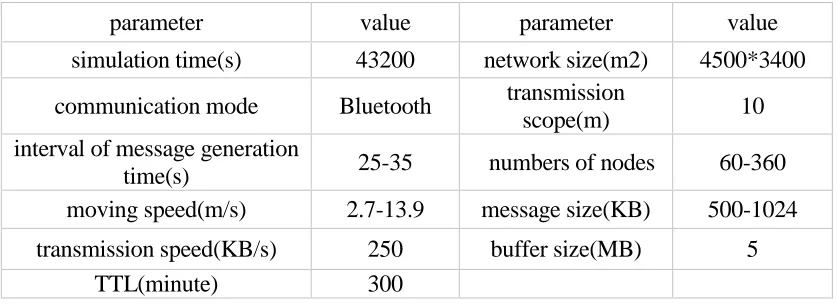
[image:4.612.89.508.553.705.2]The ONE (Opportunistic Network Environment) based on JAVA is used as the experimental platform. Each node moves according to the movement model RWP [11]. Detailed simulation parameters are set as shown in Table 1.
TABLE 1. SIMULATION PARAMETER SETTING.
parameter value parameter value
simulation time(s) 43200 network size(m2) 4500*3400
communication mode Bluetooth transmission
scope(m) 10
interval of message generation
time(s) 25-35 numbers of nodes 60-360
moving speed(m/s) 2.7-13.9 message size(KB) 500-1024
transmission speed(KB/s) 250 buffer size(MB) 5
Simulation performance analysis
[image:5.612.153.440.110.240.2]Message delivery rate
Figure 1. The influence of the node density to delivery probability.
The experiment shows: as the number of nodes increases, the delivery rates of the four routing protocols increase. The performances of Epidemic and PRoPHET are very unsatisfactory, and the delivery rate is not more than 10%. The BPAS greatly improves the delivery rate by optimizing the estimation of the encounter probability. However, the BPAS does not consider the buffer of nodes, and it may cause the nodes to drop messages because of insufficient buffer. In addition, the BPAS does not consider the order of the messages, and the real valuable message is shelved. In contrast, the FSNUV, when optimizing the encounter probability, takes into account meeting interval time between nodes and the buffer status and the next hop node is selected according to the node utility value. In addition, the FSNUV introduces the message value model, which improves the message delivery rate.
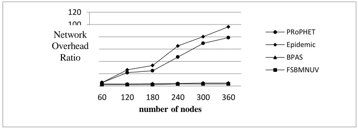
The network overhead ratio
Figure 2. The influence of the node density to overhead ratio.
The experiment shows: the network overhead ratios of FSNUV and BPAS are much lower than the Epidemic protocol and PRoPHET protocol, because FSNUV protocol and BPAS protocol can effectively control the forwarding times of messages and avoid unnecessary network overhead by using the encounter probability. In addition, FSNUV introduces the message value, so the network overhead ratio of FSNUV is the smallest of them.
0 0.2 0.4 0.6 0.8 1
60 120 180 240 300 360 number of nodes
PRoPHET Epidemic BPAS FSBMNUV
0 20 40 60 80 100 120
60 120 180 240 300 360 number of nodes
PRoPHET Epidemic BPAS FSBMNUV
Message Delivery Rate
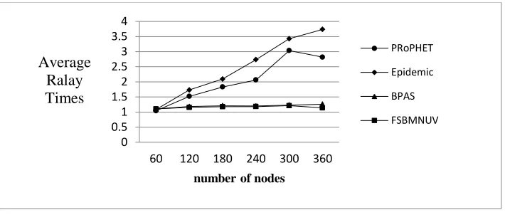
[image:5.612.113.480.464.595.2]The average relayed times
Figure 3. The influence of the node density to average relayed times.
The experiment shows: with the node density increases, the average relayed times of FSNUV is less than that of Epidemic and PRoPHET which are based on flooding. This is because FSNUV uses the node utility value model to select the next hop. In addition, a message value model is used to sort the message sending queues. The FSNUV effectively controls the average relayed times. BPAS protocol due to the lack of consideration of buffer of node and message forwarding order, therefore, the average relayed times of FSNUV are still less than that of BPAS protocol.
SUMMARY
In this paper, FSNUV is proposed that is based on the optimization of the encounter probability, considering the change rate of node, the transmission capacity of node and the connection capacity of node, node utility value model is established. FSNUV can improve the delivery probability, reduce the network overhead radio and average relayed times, so as to solve the problems of low delivery rate of routing protocols based on probability in opportunistic networks.
REFERENCES
1. Zhang Z. Opportunistic routing in mobile ad hoc delay-tolerant networks (DTNs) [J]. Advances in Delay-Tolerant Networks (DTNs), 2015(8):159-172.
2. Wen H, Ren F, Liu J, et al. A Storage-Friendly Routing Scheme in Intermittently Connected Mobile Network [J]. IEEE Transactions on Vehicular Technology, 2011, 60(3):1138-1149.
3. Wang Y, Jain S, Martonosi M, et al. Erasure-coding based routing for opportunistic networks[C]// ACM SIGCOMM Workshop on Delay-Tolerant NETWORKING. ACM, 2005:229-236.
4. Xiong Y P, Sun L M, Niu J W, et al. Opportunistic networks [J]. Journal of Software, 2009, 20 (1):124-137.
5. Lindgren A, Doria A. Probabilistic routing in intermittently connected networks [J]. Acm Sigmobile Mobile Computing & Communications Review, 2003, 7(3):19-20.
6. Du Q W, Tang R. ED_PRoPHET: an Oppportunistic routing Protocol Consider the Encounter Time[J]. Journal of Chinese Computer Systems, 2014: 35(2):282-285.
7. Zhang Y, Zhou S W. Opportunistic Networks Routing Protocol Based on Historical Intervals of Contacts [J]. Computer Engineering, 2011, 37 (14):85-87.
8. Gong D. Evaluated Probability with Information of Meeting for Opportunistic Networks Routing Procol [J]. Bulletin of Science & Technology, 2014, 30(11): 81-84.
9. Lindgren A, Doria A. Probabilistic routing in intermittently connected networks [J]. ACM Sigmobile Mobile Computing and Communications Review, 2003, 7(3):19-20.
0 0.5 1 1.5 2 2.5 3 3.5 4
60 120 180 240 300 360 number of nodes
PRoPHET
Epidemic
BPAS
FSBMNUV Average
10. Li X L, Xuan M Y. Opportunistic Network Routing Protocol Based on Messages Value[J], Journal of Chinese Computer Systems, 2016, 37(12):2603-2606.