1
Measurement and Control Systems for an Imaging Electromagnetic
Flow Meter
Y. Zhao
1,2, G. Lucas
1, T. Leeungculsatien
1and T.Zhang
2Abstract-Electromagnetic flow meters based on the principles of Faraday’s laws of induction have been used successfully in many industries. The conventional electromagnetic flow meter can measure the mean liquid velocity in axisymmetric single phase flows. However, in order to achieve velocity profile measurements in single phase flows with non-uniform velocity profiles, a novel Imaging Electromagnetic Flow meter (IEF) has been developed which is described in this paper. The novel electromagnetic flow meter which is based on the ‘weight value’ theory to reconstruct velocity profiles is interfaced with a ‘Microrobotics VM1’ microcontroller as a stand-alone unit. The work undertaken in the paper demonstrates that an imaging electromagnetic flow meter for liquid velocity profile measurement is an instrument that is highly suited for control via a microcontroller.
Helmholtz coil, induced voltage, weight value, microcontroller
I. INTRODUCTION
Electromagnetic flow meters have been used for several decades, with the basic principles being derived from Faraday’s laws of induction. Conventional 2-electrode electromagnetic flow meters (EMFMs) have been used successfully in a variety of industries for measuring volumetric flow rates of conducting fluids in single phase pipe flows. At present, a conventional 2-electrode EMFM can measure the volumetric flow rate of a single phase flow with relatively high accuracy (about
0.25% of reading) provided that the velocity profile is axisymmetric [1]. However highly non-uniform velocity profiles are often encountered, e.g. just downstream of partially open valves. The axial flow velocity just downstream of a gate valve varies principally in the direction of the valve stem, with the maximum velocities occurring behind the open part of the valve and the minimum velocities behind the closed part of the valve. In such non-uniform velocity profiles the accuracy of the conventional EMFM can be seriously affected [2-3]. One method for improving the accuracy of the volumetric flow rate estimate is to measure the axial velocity profile with the ‘Imaging Electromagnetic Flowmetering’ (IEF) technique described in this paper and then to use this profile to determine the mean flow velocity in the cross section. Previous researchers e.g. [4], [5], [6] and [7] have proposed techniques to obtain velocity profiles in the flow cross section but few practical devices have emerged. In view of the above, the main objective of this paper is to describe a new non-intrusive electromagnetic flow metering technique for measuring the axial velocity profile of single phase flows of conducting fluids. In Section III of this paper the mechanical and electrical designs of an IEF device are described, as well as the relevant signal detection and processing methods.In Section IV of the paper, a microcontroller is introduced as the processing core of the IEF to achieve the functions of
driving the magnetic field, acquiring voltage data from the electrode array, matrix inversion to calculate the velocity profile and data display.
Section V presents experimental results of local axial velocity distributions obtained from the IEF device under a variety of different flow conditions and includes comparisons with reference local axial velocity measurements obtained from a Pitot-static tube.
II. BACKGROUND THEORY
An alternative approach to accurate volumetric flow rate measurement in highly non-uniform single phase flows was proposed by authors such as Horner [8] who described a six electrode electromagnetic flow meter which is insensitive to the flow velocity profile. However, this type of flow meter cannot provide information on the local axial velocity distribution in the flow cross section unlike the IEF device presented in this paper.
The essential theory of EMFMs states that charged particles in a conducting material which move in a magnetic field experience a Lorentz force acting in a direction perpendicular to both the material’s motion and the applied magnetic field. Williams [9] applied a uniform transverse magnetic field perpendicular to the line joining the electrodes and the fluid motion and his experiments revealed that for a uniform velocity profile the flow rate is directly proportional to the voltage measured between the two electrodes. Subsequently Shercliff [10] showed that the local current density j in the fluid is governed by Ohm’s law in the form
) (E v B
j (1)
where is the local fluid conductivity, v is the local fluid velocity, and B is the local magnetic flux density. The expression (vB) represents the local electric field induced by the fluid motion, whereas E is the electric field due to charges distributed in and around the fluid. For fluids where the conductivity is constant (such as the single phase flows under consideration in this paper) Shercliff [10] simplified equation (1) to show that the distribution of the electrical potential in the flow cross section can be obtained by solving
) (
2 vB
(2)
For a circular cross section flow channel bounded by a number of electrodes, with a uniform magnetic field of flux density B normal to the axial flow direction, it can shown with reference to [10] that, in a steady flow, a solution to equation (2) which gives the potential difference Uj
between the jth pair of electrodes is of the form
vxyW xy dxdy
a B
Uj 2 ( , ) ( , )j
(3)
where v(x,y) is the steady local axial flow velocity at the point (x,y) in the flow cross section, W(x,y)j is a 1 School of Computing and Engineering, University of
Huddersfield, Huddersfield HD1 3DH, UK
2 Tianjin Key Laboratory of Process Measurement and Control,
so-called ‘weight value’ relating the contribution of v(x,y) to Uj and a is the internal radius of the flow channel.
Let us now assume that the flow cross section is divided into
N large regions (fig. 1(c)) and that the axial flow velocity in the th
i such region is constant and equal to vi (i.e. for
a given region the axial flow velocity does not vary within that region). Let us further suppose that N potential difference measurements Uj are made between
independent pairs of electrodes on the boundary. From these assumptions, and by discretising equation (3), the following relationship is obtained between the th
j potential difference measurement Uj and the ith steady axial velocity vi.
N
i i ij i
j vw A
a B U
1
2
(4)
Here Ai represents the cross sectional area of the ith
region and the term wij is the weight value which relates
the steady flow velocity in the th
i region to the th j
potential difference measurement. Provided that the required
2
N weight values are known [11] equation (4) can be manipulated to enable the steady axial flow velocity vi in
each of the N regions to be determined from the N
potential difference measurements Uj (j1 toN) made on
the boundary of the flow cross section. This process for calculating the velocity in each of the regions can be expressed by the matrix equation
U WA
V [ ]1
2
B a
(5)
where V is an N1 matrix containing the required velocities, W is an NN matrix containing the weight values wij, A is a diagonal matrix containing the cross sectional areas of the regions and U is an N1 matrix containing the N boundary potential difference measurements. Since many pipe flows are turbulent the question now arises as to what is meant by a ‘steady’ axial velocity vi in a given region in turbulent flow. Texts on
fluid mechanics e.g. [12] state that in a turbulent flow, when the velocity over a given ‘averaging’ time remains constant, the flow is termed steady. For the flows relevant to the present investigation this averaging time is approximately 7 seconds (see Sections III-D and IV-B). Consequently, when using the techniques described in this paper the measured potential differences Uj must be averaged over at least this
time period in order for repeatable velocities vi to be
obtained from one averaging period to the next. Note that equation (4) is strictly only valid if the steady local velocity in each of the N large regions is the same everywhere in a given region. However results presented in [11] show that the techniques outlined above can be used to estimate the mean axial flow velocity in a given region even when the local velocity within that region varies by as much as ±10% of the mean value for that region.
In order to calculate the weight values wij (in Equations
(4) and (5)) a finite element (F.E.) package, COMSOL, which can numerically solve equation (2) for complex geometries was used [13]. Using this F.E. package a simulated Helmholtz coil was used to produce a magnetic field with uniform magnetic flux density B in the y
direction [11]. The condition of the simulation was that the flow channel is divided into N regions and the fluid in the
th
i region has an imposed velocity vi in the z direction
while the fluid in the remaining regions is at rest. From the potential distribution obtained from this simulation, N
potential differences Uj (j1 toN) between N electrode
pairs were calculated, allowing all of the weight values wij
associated with the th
i region to be calculated according to equation (6) (with j1 toN).
i i j
ij BvA
a U
w 1
2
(6)
The process was then repeated for each of the other (N1) regions in succession until all relevant 2
N weight values were calculated.
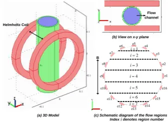
The cross section of the electromagnetic flow meter relevant to this paper is divided into 7 regions as shown in Fig. (1c) and hence N7.
Helmholtz Coil
(a) 3D Model (c) Schematic diagram of the flow regions
e2 e4
e3 e6
e7
e8
e9 e1
e5
e11
e14 e15
e10 e16
e12 e13
Flow channel
(b) View on x-y plane
B
1
i
2
i
3
i
4
i
5
i
6
i
7
i
i
[image:2.595.332.500.227.349.2]Index denotes region number
Fig. 1. Model of Finite Element Simulation. (1(c) shows the 7 regions and the boundary electrodes denoted e1 to e16)
Table 1 shows the electrode pairs between which the potential difference measurements Uj (j1 to7) are made.
The calculated weight values for a given region (index i) and for a given electrode pair (index j ) are shown graphically in Fig. (2). Note that for the case of electrode pair e1 - e9 (for which j4) the system geometry is identical to that analysed theoretically in [10]. For this geometry the local weight value W(x,y) at point (x,y) is given by
2 2
2 2
22 4
2 2 2 4
2 )
, (
x y x y a a
x y a a y
x W
(7)
By calculating the area weighted mean value of W(x,y) for each of the seven regions shown in Fig. (1) the weight values wi4 (i1 to7) can be computed and compared with
the values obtained using the numerical method described above. Fig. (3) shows the values of wi4 obtained using the
theoretical method (equation 7) and the numerical method. The good agreement between the two techniques indicates the veracity of the numerical method used in this paper for determining wij. This agreement has also previously been
reported in [14]. (Note that the value of W(x,y) tends to infinity for xa,y0 and so, when calculating w44,
Table 1: Electrode pairs between which the N potential difference measurements were made
j
U Electrode pair
j=1 e4 – e6
j=2 e3 – e7
j=3 e2 – e8
j=4 e1 – e9
j=5 e16 – e10
j=6 e15 – e11
[image:3.595.63.288.63.283.2]j=7 e14 – e12
Fig. 2. Weight values for the different regions (index i) and different
electrode pairs (index j).
Fig. 3. Comparison of weight values wi4 (associated with electrode
pair e1 – e9) obtained numerically and theoretically
III. THE ELECTROMAGNETIC FLOW METER
A. Electromagnetic Flow Meter Geometry
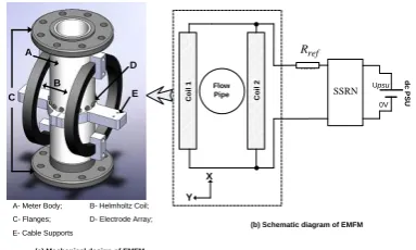
A real imaging electromagnetic flow meter (see Fig. (4a)) was constructed with the same geometry that had been modelled in the F.E. simulation described above. The non-conducting flow meter body, with an internal radius of 80mm, was made from Delrin. Four grooves on the flow meter body were accurately machined by a Computed Numerically Controlled (CNC) machine to accommodate two circular coils which formed a Helmholtz coil configuration. The Helmholtz coil consisted of a parallel pair of identical circular coils which each had the same number of turnsn.
The electrical resistances for coil1 and coil2 were each measured and both were found to be equal to 34.98Ω. At any instant in time the electrical current in each coil had the same magnitude and direction. Driving the coils in parallel (see Figs. 4 and 6) rather than in series means that, for a given supply voltage Upsu, twice the coil current and
hence twice the magnetic flux density in the flow cross section is achieved. Provided that the coils are well matched, driving them in parallel has minimal implications for the uniformity of the magnetic field.
A- Meter Body;
E- Cable Supports
d
c
P
S
U
C
o
il
2
Flow Pipe
Rref
X
Y
0V
psu
U
B- Helmholtz Coil;
D- Electrode Array; C- Flanges;
C
o
il
1
(a) Mechanical design of EMFM
(b) Schematic diagram of EMFM A
E D
C B
ref R
SSRN
Fig. 4. The IEF device used in the experiments
The mean spacing between the two coils was equivalent to
R, the mean radius of each coil, and so, at any instant in time, a near-uniform magnetic field in the y direction (see Figs. 1 and 4) existed in the flow cross section. At the plane of the electrode array ( z0 ) the components of the magnetic field in the x and z directions were always negligible. The magnitude B of the magnetic flux density of the Helmholtz coil in the y direction can be approximated by
R ni
B 0 c
5 . 1
5 4 5 .
0
(8)
where 0 is the permeability of free space and ic is the
total coil current as shown in Fig. 6. Thus B is proportional to the total coil current ic and so we may write
c
Ki
B (9)
where
R n
K 0
5 . 1
5 4 5 .
0
(10)
For the IEF device described in this paper the mean radius R of each coil was 115mm and the number of turns n
was 1024 so that when the total coil current was 2A, the magnitude of the magnetic flux density at the midpoint of the line joining the centres of the two coils was predicted to be 80gauss. Measurements obtained using a gaussmeter showed that the actual magnetic flux density (in the y
direction) at this position was 80.64 gauss.
The distribution of the y component of the magnetic flux density in the flow cross-section at the plane z0 measured using the gaussmeter is presented in Fig. 5. The maximum and minimum values of magnetic flux density were 80.68 gauss and 79.65 gauss respectively. The area weighted mean value was 80.07 gauss. This meant that the maximum variation of the magnetic flux density from the mean value was +0.76% to -0.52%. The standard deviation of the magnetic flux density in the flow cross section was 0.18 gauss. Such values are typical for ‘uniform field’ electromagnetic flow metering devices.
The electrode array contains 16 electrodes for measuring flow induced potential differences as described above, with each electrode being made from 316L stainless steel. Stainless steel was chosen for the electrode material because (i) it has high corrosion resistance and (ii) it has a low relative permeability (r1). If a corrosive material were used for the electrodes, rust could form which would reduce the electrical conductivity of the electrodes or even completely insulate them. This would create a major problem in accurately measuring the potential differences
j
[image:3.595.64.283.325.438.2]meant that they did not significantly affect the uniformity of the magnetic field in the flow cross section produced by the Helmholtz coil. Supports (‘E’ in Fig. 4(a)) were used to position the cables which run between the electrodes and the detection circuitry. These cables were mounted in such a way that they were always parallel to the local magnetic field. This meant that any ‘cable loops’ were not cut by the time varying magnetic field, thus preventing ‘non-flow-related’ potentials from being induced in the cables.
Fig. 5. Distribution of the y component of the magnetic flux density in
the flow cross-section
B. Application of a Time Dependent Magnetic Field to the Flow Cross Section
[image:4.595.69.281.447.515.2]A dc power supply unit, ‘dc PSU’ in Fig. 6, was connected to a solid state relay network (SSRN). The solid state relays were connected to form an ‘H-bridge’ configuration and two outputs from the microcontroller were used as logic inputs to the SSRN in such a way that at any instant in time the voltages applied at points ‘a’ and ‘b’ in
Fig. 6 were as per the table 2 below.
Fig. 6. Schematic diagram of coil excitation and temperature
compensation circuits
Table 2: Relay State and Voltage across Helmholtz Coil
Relay State Voltage at ‘a’ Voltage at ‘b’
RP1 Upsu 0
RP2 0 Upsu
RP3 0 0
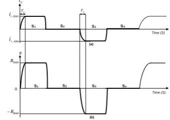
When the voltage at a was Upsu and the voltage at b
was 0 then, after all transients had died away, the maximum total coil current ic,max flowed in the coils (see Fig. 7(a)). When the voltage at a was 0 and the voltage at b was
psu
U then, after all transients had died away, the minimum
coil current ic,min flowed in the coils (where
max , min
, c
c i
i ). When the voltages at a and b were both
0, no current flowed in the coils. Thus, the variation of ic
with time was the ‘hybrid’ square wave pattern shown in Fig. 7(a). The resultant time dependent magnetic flux density in the y direction in the flow tube at z0 (the plane of the electrode array) is shown in Fig. 7(b). The reason for setting the magnetic flux density as a time dependent hybrid square
wave was (i) to reduce electrochemical effects at the electrodes and (ii) to enable the flow induced potential differences Uj to be distinguished from time dependent,
non flow induced bias voltages as described in detail in Section III-D.
The two coils were closely matched and the resistance
c
R of each coil had a known value of Rc,15 when the coils
were at a temperature of 15°C. However ambient temperature variations, and heating of the coils due to the coil current, caused the value of Rc to vary with time. The
flow induced voltages Uj from which the flow velocity
profile was reconstructed were proportional to Bmax the
maximum value of the time dependent magnetic field. In turn, Bmax was proportional to ic,max as indicated by equations (9) and (10).
Accurate velocity profile reconstruction relies upon knowing Bmax at all times and so it was necessary to know
max ,
c
i at all times. As can be seen from Fig. 6 the total coil current ic was passed through a precision reference resistor
with known resistance Rref of 0.1Ω and a very low
temperature coefficient of 20ppm/°C. A voltage Ur
appeared across Rref and was fed to the microcontroller
via a differential amplifier with a gain of 10 (‘DA’ in Fig. 6).
r
U was measured by the analogue to digital converter within
the microcontroller. The maximum value of Ur was
max , r
U where
max , max
, ref c
r R i
U (11)
Since Rref was known and Ur,max was measured by the microcontroller, ic,max could be calculated from equation (11), enabling Bmax to be calculated from equations (9) and (10) - thereby enabling the true value of the maximum magnetic field strength to be known at all times and used in the velocity reconstruction calculations.
0 S1 S2 S3 S4
B
Time (S)
c i
max ,
c
i
Time (S)
(a)
(b)
S1 S2 S3 S4
c
c
min ,
c
i
max
B
max
B
Fig. 7. (a) Variation of coil current with time over one excitation cycle
and (b) variation of the magnetic flux density with time (as measured by
a gauss meter) over one excitation cycle
The transients appearing in the coil current cycle (Fig. 7(a)) were due to the RL time-constant of the Helmholtz coil. When the relays in the SSRN were put into states RP1 or RP2 (Table 2) the current flowing through the coils could not change instantaneously. The time c required for the
current to make a change from 0 to the maximum value
max , c
i was determined by the RL time-constant of the
circuit comprising Rrefand the resistances and inductances
of the two coils (see Fig. 6).
The value of c was found to be 0.0118s, after which
the coil current ic and magnetic flux density B were both
steady (refer to Fig. 7(b)). After the microcontroller sent
c
i
+ -DA
Coil 1
SSRN
dc PSU
a b
V
0 Upsu
ref R c
i ic
Coil 2
c1 R Lc1
S
S
R
1
S
S
R
2
S
S
R
3
S
S
R
4
c2 R Lc2 DAC0
DAC1
M
ic
ro
c
o
n
tr
o
lle
r
[image:4.595.329.500.466.587.2]control signals to the relays to change the coil current ic,
the controller would wait for 0.125s to allow completion of the magnetic field transient before starting acquisition of the flow induced potential differences. This ensured that the flow induced potential differences were collected during that part of the cycle when the magnetic flux density was constant.
C. Electronic Circuit Design for Measuring the Boundary Potential Differences
A time dependent flow induced potential difference U*j
appeared between the jth electrode pair caused by the
interaction of the flowing fluid and the imposed magnetic field. A voltage Uj necessary for reconstructing the
velocity profile must be extracted from U*j using
appropriate signal processing techniques, as described later in this section.
Each pair of electrodes between which it was necessary to obtain a value of Uj was connected to the inputs of a
[image:5.595.68.288.306.365.2]separate ‘Voltage Measurement and Control Circuit’ as shown in Fig. 8.
Fig. 8. Schematic diagram of voltage measurement and control circuit
Because the applied magnetic field varies with time (as described in the previous section) U*j also varied with time.
Typically the amplitude of U*j was only a few millivolts
and so before being sampled by the ADC (analogue to digital convertor) in the microcontroller it had to be amplified by a high gain differential amplifier (HGA in Fig. 8) with gain A (equal to 996 in the present investigation). A voltage follower and a first order high pass filter (VF and HPF respectively in Fig. 8) were used to condition the signals from each electrode prior to being passed to the HGA. The high pass filters had a -3dB frequency of 0.0017Hz and a pass band gain of 1 and were used to help eliminate the very large dc offset voltages which appeared on each electrode due to the effects of the electrode/electrolyte interaction and due to the accumulation of charge on the non-conducting pipe wall. However, despite the high pass filters, the differential voltage at the input to HGA consisted of the sum of U*j and a residual, unwanted, time dependent
bias voltage U0 (Fig. 8). [Note that both U*j and U0
were differential voltages appearing across the inputs to HGA]. U0 arose as a result of electrochemical interaction between the electrodes and the process fluid (water) [15]. The magnitude of U0 was generally much larger than the amplitude of U*j.
D. Compensating for the effects of the bias voltage U 0 If the effects of U0 were not eliminated then the voltage
j x
U , measured (for the jth electrode pair) at point x in Fig.
8, would be given by Ux,jA(U0U*j) and the resultant (slowly varying) component AU0 would make the value of
j x
U , lie well outside of the range of the analogue to digital
converters on the microcontroller [note that LPF1 in Fig. 8 is a second order low pass filter with a -3dB frequency of
15.92Hzand a pass band gain of 1 and is used to eliminate any high frequency noise on the output from HGA]. The purpose of the control circuit in Fig. 8 was to compensate for the effects of U0 by continually applying a suitable control
voltage Uref to the offset input y of the HGA in such a way as to ensure that the measured output voltage Ux,j was
always of the form UxjAUjUsp *
, , where Usp is a
desired set-point dc voltage provided by the ‘set-point adjust’ unit (SPA in Fig. 8). [Note that the HGA does not amplify signals applied at the offset input y]. A suitable value for Usp could, if required, be zero. The appropriate
value for the control voltage Uref was achieved in the following way. Ux,j was low pass filtered by LPF2 (a
second order filter with a -3dB frequency of 0.28Hz and a pass band gain of 1) to remove the flow induced component
* j
AU so that only a slowly varying non flow induced component remained. The set point voltage Usp was
subtracted from this slowly varying component at the differential amplifier DA1 (Fig. 8) to give an error signal
) (t
e which was then fed to the inverting input of an integrator with a time-constant of 1 second (Fig. 8). The output voltage from the integrator was Uref, the control voltage applied to HGA.
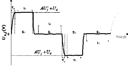
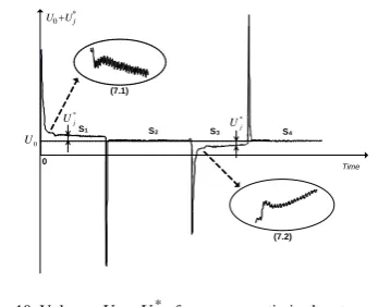
Fig. 9. Measured time dependent voltage Ux,j (when Usp0)
For the integrator time constant of 1 second, the mean value of Ux,j could be maintained steady at approximately the
set-point value Usp, irrespective of the value of U0. The variation of Ux,j with time for a given electrode pair over
a single magnetic field excitation cycle is shown in Fig. 9. For clarity in Fig 9 Usp is shown as zero. Unfortunately,
despite the presence of the control circuit, experimental observation showed that a small time dependent ‘offset’ voltage U (typically of the order of a few millivolts) was present in the signal Ux,j. U almost certainly arose from
the fact that the control circuit could not always fully restore the mean value of Ux,j to the set point voltage before the
relevant samples of Ux,j were taken (as described below).
The influence of U was eliminated as described below. It can be seen that for a single excitation cycle Ux,j can be
split into four segments (or stages) denoted S1 to S4 in Fig. 9. For stage S1, which is of length 0.3s and which corresponds to relay state RP1 in Table 2, the value of Ux,j
after transient time
c is denoted (Ux,j)1 where
U U AU Ux,j)1 j sp
( (12)
and where Uj is the maximum value of the flow induced
voltage during the excitation cycle. During the time interval of 0.175s denoted t1 in Fig. 9, the microcontroller is used to obtain an average value (Ux,j)1 from 10 samples of
1 , )
(Uxj . Note that this process is repeated for j1 to7.
DA 1
Integrator HPF
LPF 1
Feedback
Control Circuit
*
0 Uj
U
) (UxjAUjUsp
* ,
Measurement Point
HGA
+
- +
-x
j x
U,
sp
U
y ref
U
Electrode Pairth
j
Voltage Measurement Circuit VF
VF
LPF 2
HPF
-+
e(t)
GND I
C RI
[image:5.595.312.527.328.441.2]For stage S2 of the excitation cycle (which is of length 0.4s and which corresponds to relay state RP3 in Table 2), after the transient in Ux,j is completed, the value of Ux,j
is denoted (Ux,j)2 where
U U Ux,j)2 sp
( (13)
During a time interval of 0.275s, denoted t2in Fig. 9, the microcontroller is used to calculate an average value
2 , )
(Uxj from 15 samples of (Ux,j)2 for each value of j
(j1 to7).
For stage S3 of the excitation cycle (which is of length 0.3s and which corresponds to relay state RP2 in Table 2) the value of Ux,j after transient time c is denoted
3 , )
(Uxj where
U U AU Ux,j)3 j sp
( (14)
and where Uj is the minimum value of the flow induced
voltage during the excitation cycle. During a time interval of 0.175s denoted t3 in Fig. 9, the microcontroller is used to
obtain an average value (Ux,j)3 from 10 samples of
3 , )
(Uxj for each value of j (j1 to7).
Finally, for stage S4 of the excitation cycle (which is again of length 0.4s and which again corresponds to relay state RP3 in Table 2) and after the transient in Ux,j is
completed, the value of Ux,j is denoted (Ux,j)4 where
U U
Ux,j)4 sp
( (15)
During a time interval of 0.275s denoted t4 in Fig. 9 the microcontroller is used to calculate an average value (Ux,j)4
from 15 samples of (Ux,j)4 for each value of j
(j1 to7).
For the given excitation cycle the values of Uj
(j1 to7) required for calculating the velocities (see section II) are given by
A
U U U
U
Uj xj xj xj xj 2
) ( ) ( ) ( )
( , 1 , 2 , 3 , 4
(16)
Examination of equation (16) shows that the influence of
U on the values of Uj is effectively eliminated.
Furthermore, subtraction of (Ux,j)2 from (Ux,j)1 and
subtraction of (Ux,j)4 from (Ux,j)3 in equation (16) helps
to minimise the influence of the time dependent changes in
U on Uj.
From equations (12)-(15) it is apparent that equation (16) is also equivalent to the following expression
2 / ) (
j j
j U U
U (17)
where Uj and Uj are respectively the mean values of the
maximum and minimum flow induced voltages during the excitation cycle. Note that time intervals t2 and t4 (see Fig. 9) were longer than time intervals t1 and t3. This is because experimental observation showed that more noise was present on Ux,j during excitation stages S2 and S4 and
so a larger number of samples were taken to average out this noise. Note that further experimental work may be necessary to optimise the durations of stages S1 to S4 for flow conditions different to those discussed later in this paper.
Finally in this section, it is instructive to discuss the signal
*
0 Uj
U appearing at the input to the high gain differential amplifier HGA in Fig. 8 for an improperly designed IEF flow meter and for non-optimised voltage measurement and control circuitry. Under such circumstances the signal
*
0 Uj
U can appear as shown in Fig. 10. The large spikes in Fig. 10 are ‘non flow induced’ voltages arising from changes
in the magnetic flux through the loop formed by the cables connecting the electrodes to the measurement circuitry (note that the loop is completed by the conducting fluid between the relevant electrode pair). Large voltage spikes such as these can be eliminated by ensuring that the plane of each cable loop is always parallel to the local direction of the magnetic field as described in section III-A. In Fig. 10, during stages S1 and S3 of the excitation cycle, it can be seen that the flow induced voltage component may decay slightly with time. This decay can be eliminated by ensuring that the time constants of the high pass filters shown in Fig. 8 are adequately large.
Two other features of Fig. 10 are worthy of comment. (i)
Although the magnitude of the random, slowly varying, bias
voltage U0 is shown in Fig. 10 as being of the same order
of size as the amplitude of the flow induced component U*j,
in reality the magnitude of U0 could be many times greater
than the amplitude of U*j. (ii) Some high frequency noise
was always present in the flow induced signal U*j, possibly
due to flow turbulence generated at the electrodes. This high
frequency noise was eliminated by the low pass filter LPF1
placed between the high gain differential amplifier HGA and
[image:6.595.314.488.350.491.2]the measurement point x (as shown in Fig. 8).
Fig. 10. Voltage U0U*j from a non-optimised system
IV. AN ON-LINE CONTROL SYSTEM FOR THE IEF
DEVICE
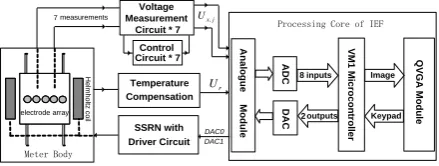
In contrast to the earliest methods employed by the authors of implementing an IEF device by processing the acquired data off-line using a PC, this section describes the use of the IEF device combined with a microcontroller as a processing core, enabling the system to work independently and to calculate and display velocity profiles on-line in real time.
A.Hardware Specification of VM1 Microcontroller
The VM1 [16] is an embedded controller which, in its use with the IEF device, is interfaced to the flow meter via an analogue I/O module as shown in Fig. 11. This Analogue Module was used to acquire the voltages Ux,j( j1 to7) as
described in section III and the voltage Ur appearing
across the reference resistance Rref (see Fig. 6) using a 12
bit analogue to digital convertor. The analogue I/O module was also connected to the SSRN so that the outputs DAC0 and DAC1 were used to control the switching of the relays SSR1 to SSR4 as shown in Fig. 6. A display panel on the VM1 enabled display of the imaged velocity profile. The
0 Time
S1 S2 S3 S4
* 0Uj
U
(7.1)
(7.2)
0
U
*
j
U *
j
LCD display was also used for display of numerical results such as totalised flow rate.
Fig. 11. Schematic diagram of IEF microcontroller processing module
B. Procedure for Controlling Operation of the IEF Device
In the embodiment of the IEF device shown in Fig. 11, before the flow meter starts running, the number of magnetic field excitation cycles G (where G5 in the present investigation) over which it is required to find the mean velocity in each region is input to the microcontroller. After each G excitation cycles the graphical and numerical displays on the LCD panel are updated (note: a single excitation cycle consists of the magnetic field undergoing stages S1 to S4 as shown in Fig. 7). Once the virtual key ‘Start’ on the touchscreen is pressed the IEF device starts working continuously. At the beginning of each stage of the excitation cycle, the VM1 sends control signals via its outputs DAC0 and DAC1 to the solid state relay network SSRN in order to generate the appropriate magnetic field. [Note that although the DAC outputs were used to operate the relay network, two of the digital I/O lines on the VM1 would have been equally satisfactory]. Measurements of
j x
U , ( j1 to7) are made by the microcontroller using the analogue to digital converters. At the first stage (S1) of each excitation cycle the SSRN is set to state RP1 (see Table 2). After the appropriate time delay, 10 samples of the induced voltages (Ux,j)1(j1 to7) and 10 samples of the voltage
1 )
(Ur across the high-precision resistance
R
ref areobtained. Mean values (Ux,j)1(j1 to7) of the induced voltages and a mean value (Ur)1 of the voltage across the
precision resistance are calculated as follows:
10 / ) ( ) ( 10 1 1 , 1 ,
q q q j x j x U U (18) 10 / ) ( ) ( 10 1 1 1
q q q r r UU (19)
This process is repeated for steps S2, S3 and S4 of each excitation cycle to generate values for (Ux,j)2, (Ux,j)3
and (Ux,j)4( j1 to7) (where for (Ux,j)2 and (Ux,j)4 equation (18) is modified to account for the fact that the averages were taken from 15, rather than 10, samples). The process is also repeated to obtain values for (Ur)2, (Ur)3
and (Ur)4.
The index for a given excitation cycle is denoted g. After each excitation cycle, mean flow induced potential differences Uj,g( j1 to7) are calculated using
A
U U
U U
Ujg xj xj xj xj
2 ) ( ) ( ) ( )
( , 1 , 2 , 3 , 4 ,
(20)
Furthermore, a mean value (Ur,max)g for the maximum
voltage drop across the precision resistance is calculated using 2 ) ( ) ( ) ( ) ( )
( ,max 1 2 3 4
r r r r g r U U U U U (21)
Note that in equation (20), A is the gain of high gain differential amplifier (HGA) shown in Fig. 8. After G
excitation cycles, the potential differences Uj ( j1 to7),
from which the velocities are reconstructed (see section II), are calculated using
G U U G g g j j / 1 ,
(22)Furthermore, after G excitation cycles, the value Ur,max
of the voltage appearing across the reference resistance (which is used in determining the magnetic flux density
max
B , using equations (9),( 10) and (11)) is calculated from
G U U G g g r
r ( ) /
1 max , max ,
(23)By setting G5, since each excitation cycle was 1.4 seconds, the axial velocity in each region was calculated from data obtained over a 7 second period. A 7 second period was experimentally found to be sufficient to enable repeatable flow velocity profile measurements to be obtained at a constant value of the reference water flow rate obtained from a turbine flow meter (see section V). Using the weight values wij ( j1 to7 , i1 to7 ) stored in the
microcontroller in array W, the cross sectional areas of the regions stored in array A , the measured potential differences Uj (j1 to7) and by setting BBmax (where
max
B is obtained as described above) the velocities vi
(i1 to7) can be calculated by solving matrix equation (5). Next, in a single phase flow, the liquid volumetric flow rate
w
Q can be calculated from the velocities vi by using
equation (24) below
7 1 i i iw vA
Q (24)
Finally, the velocity in each region is displayed on the LCD screen in bar chart form to give a graphical representation of the velocity profile. Qw can also be
displayed on the LCD screen in numerical format.
V. EXPERIMENTAL RESULTS
A series of experiments was carried out on the IEF flow meter controlled by the VM1 microcontroller. When using the VM1 device, velocity profile reconstruction was performed on-line (in real time). The IEF flow meter was mounted in the 80mm internal diameter working section of a flow loop flowing single phase water of conductivity 153µScm-1. A turbine meter was placed in series with the working section of the flow loop to enable a reference measurement Qw,ref of the water volumetric flow rate to be
made. Several flow conditions were investigated, for which the IEF device was used to measure the water velocity profile, as described below.
(i) For the first flow condition the water velocity profile at the IEF flow meter was a fully developed turbulent velocity
H e lm h o ltz c o il Control Circuit * 7
2 outputs
A
D
C 8 inputs
Voltage Measurement
Circuit * 7
SSRN with Driver Circuit Temperature Compensation V M 1 M ic ro c o n tr o lle r
electrode array DA
C Q V G A M o d u le 7 measurements A n a lo g u e M o d u le
Processing Core of IEF
profile. The reference water flow rate obtained from the turbine meter was 17.46m3hr-1. The velocity profiles reconstructed using the on-line VM1 system are shown in Fig. 12(a). From Fig. 12(a) it is clear that the reconstructed velocity is approximately the same for all of the regions – a result which is to be expected from the IEF device due to the relative flatness of the fully developed, single phase, turbulent velocity profile. Note that Fig. 12 also shows results obtained from an off-line system comprising a PC and a National Instruments data acquisition card. It is clear from Fig. 12 that the results from this off-line system are virtually identical to the results from the on-line VM1 system. This result is important because most systems for imaging industrial processes require the computing power of a PC to process and display the data, whereas the techniques outlined in this paper can be performed just as well using a simple microcontroller.
A comparison was made between the total water volumetric flow rate Qw,IEF obtained from IEF device by integration
of the water velocity profile in the flow cross section (see equation 24) and reference water volumetric flow rate
ref w
Q , obtained from the turbine meter. The mean integrated value of Qw,IEFobtained from the IEF device
was 17.54m3hr-1 whilst the mean value of Qw,ref was
17.46m3hr-1. This represents an error of 0.45% in the flow rate obtained from the IEF device. This error is of the same order of size as the quoted accuracy of the reference turbine meter and therefore suggests that the IEF device is indeed capable of accurately measuring the total water volumetric flow rate by integration of the velocities vi in the flow
cross section (equation (24)).
[image:8.595.331.500.349.525.2](ii) For the second flow condition, a gate valve was mounted just upstream of the IEF device. By partially opening the valve a velocity profile was created in which the local flow velocity increased from a minimum value at the position of electrode e13 (see Fig. 1) to a maximum value at the position of electrode e5. The velocity profile reconstructed using the VM1 system for this second flow condition is shown in Fig. 12(b) from which it is clear that the reconstructed water velocity increases from a minimum value in region 7 (adjacent to electrode e13) to a maximum value in region 1 (adjacent to e5).
Fig. 12. Velocity profiles obtained using the VM1 microcontroller with
on-line reconstruction and a PC/NI system with off-line reconstruction
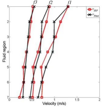
(iii) In a final experiment a flow profile conditioner comprising a bundle of tubes of different diameters was installed 200mm upstream of the IEF device to generate a velocity profile that varied from a minimum to a maximum value in the direction of increasing y . Three flow conditions f1, f2 and f3, with reference water flow rates of 16.17m3h-1, 11.55 m3h-1 and 6.93 m3h-1 (as measured by the
turbine meter), were used. The reconstructed local axial velocity distributions, at each flow condition, obtained using the IEF device (vIEF in Fig. 13) were compared with local
axial velocity distributions obtained using a Pitot-static tube
(vPitot in Fig. 13). [Note that the Pitot-static tube is a
differential pressure device used for making reference measurements of the local fluid velocity, see for example [12]]. In this experiment the Pitot-static tube was traversed to 128 different points in the flow cross section at each flow condition, allowing estimates of the mean flow velocity in each of the 7 regions (Fig. 1(c)) to be made). The magnitude of the maximum difference between vIEF and vPitot (for
all 7 regions) was 7.56%, 7% and 6.29% for flow conditions
f1, f2 and f3 respectively. Note that because the Pitot-static tube is an intrusive device, the measurements of vPitot are
likely to contain some error. More accurate measurements, for example using Laser Doppler Anemometry, may be necessary in the future to obtain a better understanding of the true accuracy of the measurements of vIEF.
[image:8.595.67.281.555.665.2]The error in the total volumetric flow rate from the IEF device (obtained using equation (24)) with respect to the reference value from the turbine meter was -0.65%, 0.90% and -0.68% for flow conditions f1, f2 and f3 respectively. This level of accuracy is sufficient for many practical flow metering applications.
Fig. 13. Comparison between measurements of the velocity downstream
of a flow profile conditioner made using the IEF device and a Pitot-static
tube.
VI. CONCLUSIONS
This paper describes a new multi-electrode electromagnetic flow meter (IEF) for imaging velocity profiles in single phase flow. A microcontroller is used as the processing core of the IEF to achieve the functions of driving the magnetic field, acquiring boundary voltage data from the electrode array, performing matrix inversion to calculate the velocity profile and displaying the calculated results in both alphanumerical and graphical format. The paper goes on to show how the IEF device can be used to map velocity profiles of both uniform and non-uniform single phase flows - such as flows behind partially open valves – and that the arrangement of the regions in which the flow velocity is measured (see Fig. 1(c)) is particularly suited to flows in which the axial flow velocity varies principally in a single direction. It has also been shown that for a fully developed turbulent flow, when the reconstructed velocities are integrated in the flow cross section to give the total liquid volumetric flow rate, the result agrees to within
(b) Valve is partially open and reference flow rate is
(a) Valve is fully open and reference flow rate is 17.46m3hr1 17.23m3hr1
Re
gi
on
s
Re
gi
on
s
0.45% with a reference measurement of the liquid volumetric flow rate obtained using a conventional turbine flow meter. For highly disturbed flows just downstream of a flow profile conditioner the error of this volumetric flow rate measurement can increase to as much as 0.9% for the range of flow conditions investigated. Measurements of local velocities obtained by the IEF device were found to agree with reference local velocity measurements obtained using a Pitot-static tube to 7.56% or better – although due to its intrusive nature measurements from the Pitot-static tube were likely to contain some error. The work presented in the paper demonstrates that a practical ‘imaging electromagnetic flow meter’ for liquid velocity profile measurement is feasible.
REFERENCES
[1] H. Kanai, “The effects upon electromagnetic flowmeter sensitivity of non-uniform field and velocity profiles,” Med.
Biol. Eng., vol. 7, no.7, pp. 661–676, 1969.
[2] K. W. Lim, M. K. Chung , “Numerical investigation on the installation effects of electromagnetic flowmeter downstream of a 90°elbow–laminar flow case,” Flow Meas. Instrum., vol. 10, pp. 167–174, Dec. 1998.
[3] A.Ono, N. Kimura, H. Kamide and A. Tobita,“ Influence of elbow curvature on flow structure at elbow outlet under high Reynolds number condition,” J. Nucl. Eng. Desi., vol. 241, pp. 4409-4419, Nov. 2011.
[4] T. Katoh and S. Honda, “3-D flow tomography through electromagnetic induction,” SICE annual conference. vol. 2, pp. 1446–1452, Aug. 2004
[5] A. Traechtler, B. Horner, and D. Schupp, “Tomographic methods in electromagnetic flow measurement for determining flow profiles and parameters,” Technisches Messen, vol. 64, no. 10, pp. 365–373, 1997.
[6] L. Xu, Y. Wang, and F. Dong, “On-Line Monitoring of Nonaxisymmetric Flow Profile With a Multielectrode Inductance Flowmeter,” IEEE Trans. Instrum. Meas., vol. 53, no. 4, pp. 1321–1326, Aug. 2004.
[7] B Horner and F Mesch “An induction flowmeter insensitive to asymmetric flow profiles,” European concerted action on
process tomography conf. (Bergen, Norway), ISBN.
0952316528, pp. 321-330, Oct. 1995.
[8] B. Horner , “A Novel profile-insensitive multi-electrode induction flowmeter suitable for industrial use,” Flow Meas.
Instrum., vol. 24, no.3, pp. 131–137, Oct. 1998.
[9] E. J. Williams, “The introduction of electromotive forces in a moving liquid by a magnetic field, and its application to an investigation of the flow of liquids,” Proc. Phys. Soc. (London), vol. A42, pp. 466-487, 1930.
[10] J. A. Shercliff, “The Theory of Electromagnetic Flow Measurement,” Cambridge, U.K.: Cambridge Univ. Press, 1962.
[11] T. Leeungculsatien and G P Lucas “Continuous phase velocity profile measurement in multiphase flow using a non-invasive multi-electrode electromagnetic flow meter,”
AIP Conf. Proc. 1428, pp. 243-250, Aug. 2011 (ISBN
978-0-7354-1011-4).
[12] B.S. Massey., “Mechanics of Fluids. 4th ed.,” Van Nostrand
Reinhold, New York, 1979
[13] COMSOL, “COMSOL Corporation Femlab 3.3 user’s guide,” 2006
[14] J Z Wang, G P Lucas and G Y Tian “A numerical approach to the determination of electromagnetic flow meter weight functions,” Meas. Sci. Technol., vol. 18, no. 3, pp. 548–554, Mar. 2007.
[15] A. C. Fisher “Electrode Dynamics,” Oxford University Press, ISBN13. 9780198556909