Munich Personal RePEc Archive
Judging statistical models of individual
decision making under risk using in- and
out-of-sample criteria
Drichoutis, Andreas and Lusk, Jayson
University of Ioannina, Oklahoma State University
19 May 2012
Online at
https://mpra.ub.uni-muenchen.de/38973/
1
Judging Statistical Models of Individual Decision Making Under Risk Using In- and
Out-of-Sample Criteria
Andreas Drichoutis† and Jayson L. Lusk‡
†
Department of Economics, University of Ioannina, Greece, email: [email protected]
‡
Department of Agricultural Economics, Oklahoma State University, USA, email:
Abstract: Despite the fact that conceptual models of individual decision making under
risk are deterministic, attempts to econometrically estimate risk preferences require some
assumption about the stochastic nature of choice. Unfortunately, the consequences of
making different assumptions are, at present, unclear. In this paper, we compare two
popular error specifications (Luce vs. Fechner), with and without accounting for
contextual utility, for two different conceptual models (expected utility and
rank-dependent expected utility) using in- and out-of-sample selection criteria. We find
drastically different inferences about structural risk preferences across the competing
specifications. Overall, a mixture model combining the two conceptual models assuming
Fechner error and contextual utility provides the best fit of the data both in- and
out-of-sample.
JEL codes: C91, C25, D81
Keywords: error specification, expected utility theory, experiment, probability
2
1. Introduction
Virtually all conceptual models of risky choice, including expected utility theory
(EUT) and the behavioral alternatives such as prospect theory, are deterministic. The
deterministic nature of the theories presents a challenge for applied economists
attempting to econometrically estimate risk preferences in a sample of individuals. In
essence, the analyst must make assumptions about the decision making process that go
above and beyond the content of the theory, making it difficult to conduct clean tests of
the underlying theory itself and to confidently identify underlying structural parameters.
While a few previous studies have analyzed the extent to which different stochastic error
specifications influence estimates of risk preferences (e.g., Hey, 2005, Loomes, 2005),
there have been new developments in the field (e.g., Wilcox, 2011) that have not been
addressed in previous model comparisons, and there has been an almost exclusive focus
on the ability of models to fit the data in-sample.
The focus on in-sample fit is particularly important in determining which decision
making theory, EUT or a behavioral alternative, best describes lottery choices. EUT is a
relatively parsimonious theory, characterizing risk preferences simply by the curvature of
the utility function over income or wealth. Some popular functional forms such as
constant relative (or constant absolute) risk aversion consist of a single parameter.
Behavioral theories often proceed by adding parameters to the basic EUT set-up.
Cumulative prospect theory, for example, allows for different degrees of curvature in the
gain and loss-domains and for additional parameters describing the extent to which
individuals under- or over-weight low probability events (both in the gain and loss
domains). Given the additional parameters, there might be a tendency for such behavioral
models to over-fit the data, and while in-sample test statistics, such as Akaike or
Bayesian Information Criteria, suggest improvements in model fit, this is no guarantee
the model will perform better predicting out-of-sample. Although several previous
studies have compared different decision making models under risk (Harless and
Camerer, 1994, Hey and Orme, 1994), and Carbone and Hey (2000) have attempted to
reconcile differences between studies based on differential assumptions made about how
3
compared different error specifications and risk models insofar as their ability to predict
out-of-sample.
Because most experimental studies are performed with a relatively small sample
of subjects, it would seem that most analysts are attempting to extrapolate risk
preferences sample to the more general population, and as such, studying
sample prediction performance appears a worthwhile line of inquiry. Judging
out-of-sample prediction performance is not always easy for discrete choice problems, and as
such, we turn to the out-of-sample-log-likelihood function approach long used in the
marketing literature for model selection (Erdem, 1996, Roy et al., 1996) and further
elucidated in the economics literature by Norwood et al. (2004a, 2004b).
The purpose of this paper is to use several in- and out-of sample model selection
criteria to determine which stochastic error specification and theoretical model best fits
lottery choice data gathered in an experimental setting. In particular, we compare two
different error specifications (Luce vs. Fechner), with and without accounting for
Wilcox’s (2011) contextual utility specification, for two different conceptual models
(EUT and rank-dependent EUT) using in- and out-of-sample selection criteria.
Moreover, we further investigate Harrison and Rutström’s (2009) claim that a combined
model (combining EUT and rank-dependent EUT) leads to improved inferences.
The next section of the paper describes the laboratory experiment we conducted to
elicit preferences for competing lotteries. Then, we describe the competing approaches
used to estimate risk preferences, after which we present the results from the competing
models. Following this discussion, we discuss different model selection criteria and
indicate the best fitting models. The last section concludes.
2. Experimental procedures
2.1.Description of the experiment
A conventional lab experiment was conducted using z-Tree software (Fischbacher,
4
and were recruited using the ORSEE recruiting system (Greiner, 2004). During the
recruitment, subjects were told that they would be given the chance to make more money
during the experiment.1
Subjects participated in sessions of group sizes that varied from 9 to 11 subjects per
session (all but two sessions involved groups of 10 subjects). In total, 100 subjects
participated in 10 sessions that were conducted between December 2011 and January
2012. Each session lasted about 45 minutes and subjects were paid a €10 participation
fee. Subjects were given a power point presentation explaining the lottery choice tasks as
well as printed copies of instructions. They were also initially given a five-choice training
task to familiarize them with the choice screens that would appear in the tasks involving
real payouts. Subjects were told that choices in the training phase would not count toward
their earnings and that this phase was purely hypothetical.
Full anonymity was ensured by asking subjects to choose a unique three-digit code
from a jar. The code was then entered at an input stage once the computerized experiment
started. The experimenter only knew correspondence between digit codes and profits.
Profits and participation fees were put in sealed envelopes (the digit code was written on
the outside) and were exchanged with digit codes at the end of the experiment. No names
were asked at any point of the experiment. Subjects were told that their decisions were
independent from other subjects, and that they could finish the experiment at their own
convenience. Average total payouts including lottery earnings were 15.2€ (S.D.=4.56).
2.2.Risk preference elicitation
We elicited risk preferences using the popular Holt and Laury (2002) multiple price
list (MPL) task, at two payout (low vs. high) amounts. The baseline H&L MPL presented
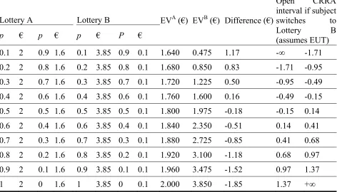
subjects with a choice between two lotteries, A or B, as illustrated in Table 1. In the first
row, the subject was asked to make a choice between lottery A, which offers a 10%
1
Subjects were told that “In addition to a fixed fee of 10€, you will have a chance of receiving additional money up to 25€. This will depend on the decisions you make during the experiment.”Stochastic fees have been shown to be able to generate samples that are less risk averse than would otherwise have been
5
chance of receiving €2 and a 90% chance of receiving €1.6, and lottery B, which offers a
10% chance of receiving €3.85 and a 90% chance of receiving €0.1. The expected value
of lottery A is €1.64 while for lottery B it is €0.475, which results in a difference of €1.17
between the expected values of the lotteries. Proceeding down the table to the last row,
the expected values of both lotteries increase, but the rate of increase is larger for option
B. For each row, a subject choose A or B, and one row was randomly selected as binding
for the payout. The last row is a simple test of whether subjects understood the
instructions correctly.2 The high payout task is identical to the control (shown in table 1)
except that all payouts are scaled up by a magnitude of five.
Instead of providing a table of choices arrayed in an ordered manner all appearing at
the same page as in H&L, each choice was presented separately showing probabilities
and prizes (as in Andersen et al., 2011)). Subjects could move back and forth between
screens if they wanted to revise their choices. Once all ten choices were made,
inaccessible no further changes were possible. In addition to the choices shown in table 1,
subjects also made a similar set of ten choices except the magnitudes of all payoffs were
scaled up by a factor of five. The order of appearance of the set of ten choices (low vs.
high payouts) for each subject was completely randomized to avoid order effects
(Harrison et al., 2005). An example of one of the decision tasks is shown in Figure 1. For
each subject, one of the choices was randomly chosen and paid out.
3. Structural estimation of risk preferences
3.1.Conceptual specification: Expected utility vs. Rank dependent utility theory
To estimate risk preferences, we follow the framework of Andersen et al. (2008). Let
the utility function be the CRRA specification:
(1)
11
r
M U M
r
2
6
where r is the CRRA coefficient and where r=0 denotes risk neutral behavior, r>0
denotes risk aversion behavior and r<0 denotes risk loving behavior.
If we assume that expected utility theory (EUT) describes subjects’ risk preference
tasks, then the expected utility of lottery i can be written as:
(2)
1,2i j j
j
EU p M U M
where p M
j are the probabilities for each outcome Mj that are induced by theexperimenter (i.e., columns 1, 3, 5 and 7 in Table 1).
Despite the intuitive and conceptual appeal of EUT, a number of experiments
suggest that EUT often fails as a descriptive model of individual behavior. Although
there are many proposed alternatives to EUT, here we consider Rank Dependent Utility
(RDU) (Quiggin, 1982), which was incorporated into Tversky and Kahneman’s (1992)
cumulative prospect theory. RDU extends the EUT model by allowing for non-linear
probabilitiy weighting associated with lottery outcomes. To calculate decision weights
under RDU, one replaces expected utility in equation (2) with:
(3)
1,2 1,2
i j j j j
j j
EU w p M U M w U M
where w2 w p
2 p1
w p
1 1 w p
1 and w1 w p
1 , with outcomes ranked fromworst (outcome 2) to best (outcome 1) and w
is the weighting function. We assume
w takes the form proposed by Tversky and Kahneman (1992):
(4)
1 1
w p p p p
When 1, it implies that w p
p and this serves as a formal test of thehypothesis of no probability weighting.
3.2.Stochastic error specification: Fechner vs. Luce
To explain choices between lotteries, one option is to utilize the stochastic specification
originally suggested by Fechner (1860/1966) and popularized by Hey and Orme (1994).
7 (5) EUF
EUBEUA
can be calculated where EUA and EUB refer to expected utilities (or rank-dependent
expected utilities) of options A and B (the left and right lottery respectively, as presented
to subjects), and where μ is a noise parameter that captures decision making errors. The
latent index is linked to the observed choices using a standard cumulative normal
distribution function
EU
, which transforms the argument into a probabilitystatement.
There are two observationally equivalent interpretations of the Fechner error
specification. The most natural, given the set-up above, is that the term μ literally
captures the effect of decision making errors on the part of the subjects. Another way to
interpret this speciation is through the random utility framework (McFadden, 1974). In
this framework, utility consists of a systematic component, EUA, observable to the
analyst, and a stochastic component, εA, unobserved by the analyst but presumed known
to the subject. In the random utility framework, the probability of choosing option A over
B is the probability that EUA - EUB > εB-εA. If the difference is distributed normally with
mean zero and standard deviation μ, then the probability of choosing A over B is given
by
EU
which, of course, is the same expression shown above.An alternative to the Fechner error specification, is the Luce error (Luce, 1959)
popularized by Holt and Laury (2002). In this case the index in (5) can be written as:
(6)
exp exp exp B L A B EU EU EU EU 3.3.Contextual utility
Wilcox (2011) proposed a “contextual utility” error specification which modifies the
Fechner and Luce error specifications, respectively as:
(7) EUCF
EUBEUA
c and(8)
exp exp exp
B CL
A B
EU c
EU
EU c EU c
8
In (7) and (8), c is a normalizing term, defined as the maximum utility over all prizes
in a lottery pair minus the minimum utility over all prizes in the same lottery pair. It
changes from lottery pair to lottery pair, and thus it is said to be contextual. The
contextual utility correction is basically a way to accommodate lottery-specific
heteroskedasticity.
3.4.Estimation
After defining the conceptual model, error specification, and contextual specification,
the conditional log-likelihood can then be written as:
(9) ln
, ; ,
ln | i 1
ln 1
| i 1
i
L r y X
Z y Z y where Z
EUj
for the Luce or the Luce with contextual utility error story (j=L, CL)and Z EUj for the Fechner or the Fechner with contextual utility error story (j=F,
CF). yi 1 1
denotes the choice of the option B (A) lottery in the risk preference task i.Subjects were allowed to express indifference between choices and were told that if that
choice was selected to be played out, the computer would randomly choose one of the
two options for them and that both choices had equal chances of being selected. The
likelihood function for indifferent choices is constructed such that it implies a 50/50
mixture of the likelihood of choosing either lottery so that (9) can be rewritten as:
(10)
ln | 1 ln 1 | 1
ln , ; , 1 1
ln ln 1 | 0
2 2
i i
i i
Z y Z y
L r y
Z Z y
XEquation (10) is maximized using standard numerical methods. The statistical
specification also takes into account the multiple responses given by the same subject and
allows for correlation between responses by clustering standard errors, which were
computed using the delta method.
Instead of discriminating between EUT and RDU models, one could allow the data
generating process to admit more than one choice models. Harrison and Rutström (2009)
allowed more than one process to explain observed behavior instead of assuming that the
9
allowed to be EUT-consistent and other choices were allowed to be Prospect
Theory-consistent (which is also equivalent to the rank dependent model in our experimental
design) and found roughly equal support. A mixture model poses a different question to
the data. As Harrison (2008) noted, “if two data-generating processes are allowed to
account for the data, what fraction is attributable to each, and what are the estimated
parameter values?”
Let EUT denote the probability that EUT is correct and RDU 1 EUT denote the
probability that the RDU model is correct. We can then replace (8) or (9) with:
(11) lnL r
EUT,rRDU, , ; ,
y X
ln
EUTLEUT
RDULRDU
.
4. Estimated risk preferences
The purpose of this section is to demonstrate the implications of different
assumptions about error specification and conceptual model, and illustrate how these
choices can lead to significantly different characterizations of risk preferences; facts
which make necessary the possibility to discriminate between models based on model fit
criteria.
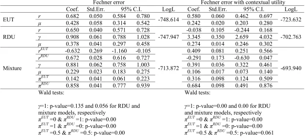
Tables 2 and 3 show the estimated parameters from the EUT, RDU and mixture
models when we assume Fechner or Luce error, with and without contextual utility. First
compare the conceptual models, EUT and RDU, under the assumption of a Fehcner or
Luce error specification without accounting for contextual utility. Results show that
subjects are on average risk averse (estimates of r span between 0.638 to 0.682) and that
the introduction of probability weighting does not have a significant effect on risk
aversion. This is mainly because the estimate for γ in the probability weighting function
of the RDU model is very close to 1. Thus in the context of EUT and RDU the choice
between a Fechner and a Luce error specification does not seem to have a substantive
effect on implied risk preferences.
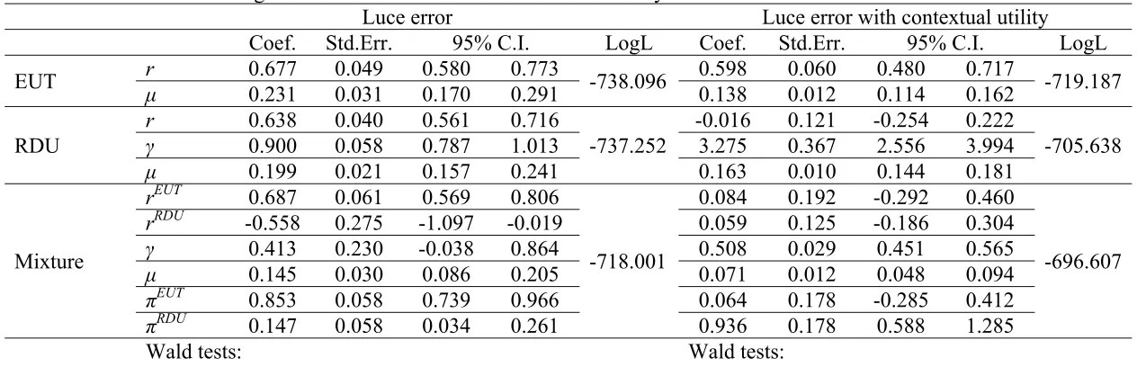
However, when we consider the mixture model with Fechner or a Luce error,
dramatically shifts in implied risk preferences occur. First note, that the mixture
probabilities πEUT and πRDU are reversed in magnitude depending on which error
10
EUT (86% by RDU) while under Luce error, roughly 85% of choices are supported by
EUT (15% by RDU). In addition, the estimated risk aversion coefficients imply risk
loving preferences for EUT and risk aversion for RDU under a Fechner error, while it is
the exact opposite for the Luce error story. Clearly, the results regarding underlying risk
preferences are highly sensitivity to assumptions about error specification, a fact which
may well cause some skepticism over previous analyses reporting a single specification.
Now we turn to the impact of contextual utility. The EUT model is least affected by
the introduction of contextual utility in both the Fechner and Luce error specification.
Although, the CRRA estimates are lower in magnitude as compared to the non-contextual
utility specifications (compare for example, the 0.58 estimate with 0.68 for the Fechner
error), the estimates still imply significant risk aversion. The most significant effects are
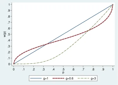
found in the RDU specifications. CRRA coefficients span around zero, implying risk
neutrality, while γ is estimated to have an unusually large value of 3. While large, this
particular value for γ, is not totally unrealistic, and Figure 2 shows it implies significant
under-weighting for all probabilities. In fact, it implies that subjects totally ignore choices
with probabilities lower than 0.2. The most commonly observed values for γ, e.g. when
γ=0.6, also imply under-weighting for probabilities larger than 0.35.
The introduction of a mixture specification not only produces different results as
compared to the non-contextual utility counterparts, but it also produces different
characterizations of risk preferences depending on whether the Fechner or Luce error are
assumed. For example, under the Fechner error, the mixture probabilities imply that
about 31.6% of all choices are EUT consistent while under the Luce error only about 6%
of the choices are consistent with EUT. Under the Fechner error, the risk aversion
coefficients imply risk aversion for EUT and risk neutrality of RDU while both CRRA
estimates under the Luce error specification span around zero implying risk neutrality.
Note that under Luce error, πEUT fails to reject the null, which implies that the mixture
model could collapse to the RDU specification. In addition, γ values are estimated at the
more commonly observed values of 0.4 and 0.5, respectively.
Taken together, the results in tables 2 and 3 demonstrate that the menagerie of error
stories that one could adopt for modeling risk preference estimation can lead to a variety
11
coefficient or relative risk aversion spans across models from a low of -0.632 (extreme
risk seeking) to a high of 0.687 (extreme risk aversion). Moreover, the estimate of the
shape of the probability weighting function under RDU goes from γ=0.391 (extreme under-weighting of low probability events) to γ=0.9 (near linear probability weighting implying EUT) to γ=3.345 (under-weighting of all probabilities) depending on what is assumed about the error and contextual utility specification. Thus, it is critically
important to be able to select between competing models based on model fit criteria.
5. Model selection criteria
5.1.Information criteria
Information criteria like the Akaike’s information criterion (AIC) and the Bayesian
information criterion (BIC) are common measures of goodness of fit; however, the
statistics do not reveal how well a model fits the data in an absolute sense, i.e., there is no
null hypothesis being tested. Nevertheless, these measures offer relative comparisons
between models on the basis of information lost from using a model to represent the
(unknown) true model.
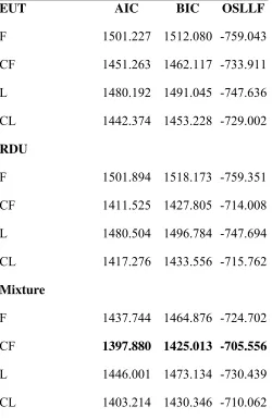
Table 4 shows that based on AIC and BIC criteria, the contextual utility specifications
are always preferred over their non-contextual utility counterpart specifications. When
comparing between EUT, RDU and the mixture specifications, AIC and BIC coincide in
indicating that the Luce error with contextual utility (for EUT) and the Fechner error
story with contextual utility (for RDU and mixture) are the error stories best fitting the
data.
When comparing between models, the mixture specification with Fechner error and
contextual utility shows the lowest AIC/BIC values.
5.2.Non-nested tests
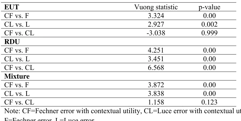
The classical approach for testing between non-nested models is the Vuong test
(Vuong, 1989). The Vuong test is a model selection test that compares between
competing models and chooses the best model based on some predefined criteria. The
12
Information Criterion (KLIC), which measures the distance between a hypothesized
likelihood function and the true likelihood function.
The null hypothesis of the Vuong test is:
(12)
0
| ;
: ln 0
| ;
i i f
i i g
f Y X
H E
g Y X
where θf and θg are parameters and f(·), g(·) are the likelihood functions of the two
competing models. The null in (12) implies that the two models are equivalent. The
alternative hypothesis favors the model with the higher average log-likelihood, if it is
significantly greater than the average log-likelihood of the competing model.
Because the Vuong test is only normally distributed asymptotically, small sample
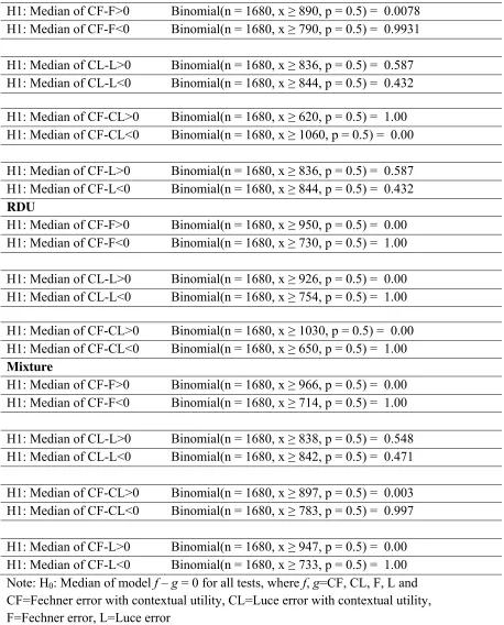
sizes may pose a problem. A non-parametric alternative to the Vuong test is the Clarke
test (Clarke, 2003). The Clarke test is a paired sign test of the differences in the
individual log-likelihoods from two non-nested models. The null hypothesis is that the
probability of the log-likelihood paired differences being greater than zero is equal to the
probability of the log-likelihood paired differences being less than zero, which in essence
is a binomial test with p = 0.5. The Clarke test is similar to the Wilcoxon sign-rank test,
but without the additional assumption that the distribution of paired differences is
symmetric.
If the models are equally close to the true specification, half the log-likelihood
differences should be greater than zero and half should be less than zero. If one model is
“better”, then more than half the log-likelihood differences should be greater than zero.
The null hypothesis of the Clarke test is:
(13) H0: median of lnf Y X
i| i;f
lng Y X
i| i;g
0Table 5 shows results from Vuong’s tests which are performed between error
specifications for the EUT, RDU and the mixture models. We first compare the errors
with contextual utility versus the errors without contextual utility. The large positive
values, and the corresponding low p-values, indicate that the null that the two competing
models are equivalent is rejected in all cases. In fact, the contextual utility specification is
favored against the non-contextual utility specification across EUT, RDU and the mixture
13
Next, we compare the Fechner and Luce error specifications with contextual utility.
The large negative value for EUT favors the Luce error while for RDU the Fechner error
is favored. For the mixture model, we fail to reject the null when we compare between
the two contextual utility specifications, although the result is marginally not significant
in favor of the Fechner error. In all, results from Vuong’s tests support the results from
the AIC and BIC model selection criteria.
Vuong’s test is suitable for non-nested models, thus we do not compare error
specifications between EUT, RDU and the mixture models since these are, by
construction, nested in each other. For example, one can test whether the mixture model
collapses to EUT or RDU by testing whether the mixture probabilities are statistically
significantly different from zero. Or one can test whether RDU collapses in EUT by
testing whether γ=1. For the Fechner error specification with contextual utility (note that
although this specification is not favored by Vuong’s test, the test marginally fails to
reject the null), Wald tests in Table 2 show that it neither collapses to either EUT or
RDU, nor does RDU in the mixture specification collapses to EUT.
Table 5 shows results from Clarke’s non-parametric test. For each model (EUT,
RDU, mixture), we first compare the contextual utility with the non-contextual utility
counterparts. Each comparison involves two, one-sided tests. For EUT, RDU and the
mixture models, the Fechner error with contextual utility is favored as compared to the
non-contextual utility counterpart. The Luce error with contextual utility is favored in the
RDU model, while Clarke’s tests show that in EUT and the mixture specification Luce
error with and without contextual utility are equivalent.
Further comparisons, show that the Fechner error with contextual utility is favored for
RDU and the mixture specifications. For EUT, Clarke’s test shows that Luce error with
contextual utility performs better than Fechner error with contextual utility, while it is
equivalent with the Luce error without contextual utility. This is an indication that
inferences that involve assumptions about transitivity between pairs of models tested may
not follow in these types of tests.
14
The out-of-sample log likelihood (OSLLF) criterion evaluates models by their fit out
of sample. In essence, the OSLLF approach uses one set of data to estimate the
parameters of the model, and then, given these parameters, calculates the likelihood
function values observed at out-of-sample observations. The OSLLF value is calculated
by using out-of sample observations to calculate the likelihood function:
(14) ˆ
|
ln
| ˆ ,
N
i f i
i i
I f Y f y
where ˆf,i is the parameter vector estimated without the ith set of observations. The
OSLLF value can be calculated in several ways (Norwood et al., 2004a). The estimate
,
ˆ
f i
could be calculated using cross-validation where ˆf,i is estimated using every
observation except i. This is referred to as “leave one out at a time forecasting.”
Alternatively, one could partition the observations into groups where each group is
iteratively omitted and ˆf,i is estimated. Then, the omitted group of observations can be
used to calculate the OSLLF. This procedure is known as grouped-cross-validation. In
what follows, we carry out group-cross validation with individuals being the partitions,
where each partition contains twenty observations (as many as the choices of the subject).
Essentially, we leave one subject (and their associated 20 choices) out at a time, estimate
the model, and calculate (14) for the subject. The process is repeated for every subject in
the sample.
Table 4 reports OSLLF values for each of the error specification for each conceptual
model (EUT, RDU and the mixture model). The results reveal that the contextual utility
specifications rank higher than their non-contextual utility counterparts across all models.
For EUT, the error specification that ranks highest is the Luce error with contextual
utility while the Fechner error with contextual utility ranks higher for RDU and the
mixture model. Across all error specifications and conceptual models, the Fechner error
with contextual utility ranks highest both in terms of OSLLF.
15
To derive estimates of individual’s risk preferences, analysts have to have some
mechanism for translating the conceptual models of risky decision making into an
empirical model that includes stochastic errors. The results presented in this paper reveal
that seemingly innocuous assumptions about this stochastic process can lead to
substantially different inferences about risk preferences. Indeed, one can estimate
parameters consistent with a high level of risk seeking or a high level of risk aversion
depending on how errors are incorporated into the statistical model; a finding which
suggests caution in naively assuming adopting a single error specification.
A battery of in- and out-of-sample model selection criteria suggest that the model that
best fits our data is an EUR-RDU mixture model assuming a Fechner error with
contextual utility. We find that 32% of the sample is characterized by EUT with a
coefficient of relative risk aversion equal to 0.4, and 68% is characterized by RDU with a
coefficient of relative risk aversion statistically indistinguishable from zero but with a
probability weighting function implying significant overweighting of low probability
16
Table 1. The H&L Multiple Price List
Lottery A Lottery B EVA (€) EVB (€) Difference (€)
Open CRRA interval if subject switches to Lottery B (assumes EUT)
p € p € p € P €
0.1 2 0.9 1.6 0.1 3.85 0.9 0.1 1.640 0.475 1.17 -∞ -1.71 0.2 2 0.8 1.6 0.2 3.85 0.8 0.1 1.680 0.850 0.83 -1.71 -0.95
0.3 2 0.7 1.6 0.3 3.85 0.7 0.1 1.720 1.225 0.50 -0.95 -0.49
0.4 2 0.6 1.6 0.4 3.85 0.6 0.1 1.760 1.600 0.16 -0.49 -0.15
0.5 2 0.5 1.6 0.5 3.85 0.5 0.1 1.800 1.975 -0.18 -0.15 0.14
0.6 2 0.4 1.6 0.6 3.85 0.4 0.1 1.840 2.350 -0.51 0.14 0.41
0.7 2 0.3 1.6 0.7 3.85 0.3 0.1 1.880 2.725 -0.85 0.41 0.68
0.8 2 0.2 1.6 0.8 3.85 0.2 0.1 1.920 3.100 -1.18 0.68 0.97
0.9 2 0.1 1.6 0.9 3.85 0.1 0.1 1.960 3.475 -1.52 0.97 1.37
17
Table 2. Estimates assuming Fechner error with and without contextual utility
Fechner error Fechner error with contextual utility
Coef. Std.Err. 95% C.I. LogL Coef. Std.Err. 95% C.I. LogL
EUT r 0.682 0.050 0.584 0.780 -748.614 0.580 0.060 0.462 0.697 -723.632
μ 0.428 0.058 0.314 0.542 0.242 0.020 0.203 0.280
RDU
r 0.650 0.040 0.571 0.728
-747.947
-0.038 0.105 -0.244 0.168
-702.763
γ 0.908 0.061 0.788 1.028 3.345 0.350 2.659 4.032
μ 0.378 0.041 0.297 0.458 0.274 0.014 0.246 0.302
Mixture
rEUT -0.632 0.269 -1.160 -0.105
-713.872
0.409 0.081 0.251 0.566
-693.940
rRDU 0.672 0.028 0.616 0.727 -0.291 0.173 -0.630 0.047
γ 0.881 0.062 0.758 1.003 0.391 0.036 0.322 0.461
μ 0.229 0.023 0.183 0.275 0.106 0.017 0.073 0.140
πEUT
0.142 0.041 0.061 0.223 0.316 0.098 0.124 0.509
πRDU
0.858 0.041 0.777 0.939 0.684 0.098 0.491 0.876
Wald tests:
γ=1: p-value=0.135 and 0.056 for RDU and mixture models, respectively
πEUT
=0 & πRDU =1: p-value=0.00
πEUT
=1 & πRDU =0: p-value=0.00
πEUT
=0.5 & πRDU =0.5: p-value=0.00
Wald tests:
γ=1: p-value=0.00 and 0.00 for RDU and mixture models, respectively
πEUT
=0 & πRDU =1: p-value=0.00
πEUT
=1 & πRDU =0: p-value=0.00
πEUT
18
Table 3. Estimates assuming Luce error with and without contextual utility
Luce error Luce error with contextual utility
Coef. Std.Err. 95% C.I. LogL Coef. Std.Err. 95% C.I. LogL
EUT r 0.677 0.049 0.580 0.773 -738.096 0.598 0.060 0.480 0.717 -719.187
μ 0.231 0.031 0.170 0.291 0.138 0.012 0.114 0.162
RDU
r 0.638 0.040 0.561 0.716
-737.252
-0.016 0.121 -0.254 0.222
-705.638
γ 0.900 0.058 0.787 1.013 3.275 0.367 2.556 3.994
μ 0.199 0.021 0.157 0.241 0.163 0.010 0.144 0.181
Mixture
rEUT 0.687 0.061 0.569 0.806
-718.001
0.084 0.192 -0.292 0.460
-696.607
rRDU -0.558 0.275 -1.097 -0.019 0.059 0.125 -0.186 0.304
γ 0.413 0.230 -0.038 0.864 0.508 0.029 0.451 0.565
μ 0.145 0.030 0.086 0.205 0.071 0.012 0.048 0.094
πEUT
0.853 0.058 0.739 0.966 0.064 0.178 -0.285 0.412
πRDU
0.147 0.058 0.034 0.261 0.936 0.178 0.588 1.285
Wald tests:
γ=1: p-value=0.082 and 0.011 for RDU and mixture models, respectively
πEUT
=0 & πRDU =1: p-value=0.00
πEUT
=1 & πRDU =0: p-value=0.011
πEUT
=0.5 & πRDU =0.5: p-value=0.00
Wald tests:
γ=1: p-value=0.00 and 0.00 for RDU and mixture models, respectively
πEUT
=0 & πRDU =1: p-value=0.721
πEUT
=1 & πRDU =0: p-value=0.00
πEUT
19
Table 4. Information criteria and out-of-sample Log-Likelihood function summary statistics
EUT AIC BIC OSLLF
F 1501.227 1512.080 -759.043
CF 1451.263 1462.117 -733.911
L 1480.192 1491.045 -747.636
CL 1442.374 1453.228 -729.002
RDU
F 1501.894 1518.173 -759.351
CF 1411.525 1427.805 -714.008
L 1480.504 1496.784 -747.694
CL 1417.276 1433.556 -715.762
Mixture
F 1437.744 1464.876 -724.702
CF 1397.880 1425.013 -705.556
L 1446.001 1473.134 -730.439
CL 1403.214 1430.346 -710.062
20
Table 5. Vuong’s non-nested tests
EUT Vuong statistic p-value
CF vs. F 3.324 0.00
CL vs. L 2.927 0.002
CF vs. CL -3.038 0.999
RDU
CF vs. F 4.251 0.00
CL vs. L 3.451 0.00
CF vs. CL 6.568 0.00
Mixture
CF vs. F 3.872 0.00
CL vs. L 3.838 0.00
CF vs. CL 1.158 0.123
21
Table 6. Clarke’s non-parametric non-nested tests
EUT
H1: Median of CF-F>0 Binomial(n = 1680, x ≥ 890, p = 0.5) = 0.0078 H1: Median of CF-F<0 Binomial(n = 1680, x ≥ 790, p = 0.5) = 0.9931
H1: Median of CL-L>0 Binomial(n = 1680, x ≥ 836, p = 0.5) = 0.587 H1: Median of CL-L<0 Binomial(n = 1680, x ≥ 844, p = 0.5) = 0.432
H1: Median of CF-CL>0 Binomial(n = 1680, x ≥ 620, p = 0.5) = 1.00 H1: Median of CF-CL<0 Binomial(n = 1680, x ≥ 1060, p = 0.5) = 0.00
H1: Median of CF-L>0 Binomial(n = 1680, x ≥ 836, p = 0.5) = 0.587 H1: Median of CF-L<0 Binomial(n = 1680, x ≥ 844, p = 0.5) = 0.432
RDU
H1: Median of CF-F>0 Binomial(n = 1680, x ≥ 950, p = 0.5) = 0.00 H1: Median of CF-F<0 Binomial(n = 1680, x ≥ 730, p = 0.5) = 1.00
H1: Median of CL-L>0 Binomial(n = 1680, x ≥ 926, p = 0.5) = 0.00 H1: Median of CL-L<0 Binomial(n = 1680, x ≥ 754, p = 0.5) = 1.00
H1: Median of CF-CL>0 Binomial(n = 1680, x ≥ 1030, p = 0.5) = 0.00 H1: Median of CF-CL<0 Binomial(n = 1680, x ≥ 650, p = 0.5) = 1.00
Mixture
H1: Median of CF-F>0 Binomial(n = 1680, x ≥ 966, p = 0.5) = 0.00 H1: Median of CF-F<0 Binomial(n = 1680, x ≥ 714, p = 0.5) = 1.00
H1: Median of CL-L>0 Binomial(n = 1680, x ≥ 838, p = 0.5) = 0.548 H1: Median of CL-L<0 Binomial(n = 1680, x ≥ 842, p = 0.5) = 0.471
H1: Median of CF-CL>0 Binomial(n = 1680, x ≥ 897, p = 0.5) = 0.003 H1: Median of CF-CL<0 Binomial(n = 1680, x ≥ 783, p = 0.5) = 0.997
22
23
[image:24.612.95.490.59.345.2]
Figure 2. Comparison of probability weighting functions for three gamma (g) values
0 .1 .2 .3 .4 .5 .6 .7 .8 .9 1
w(
p
)
0 .1 .2 .3 .4 .5 .6 .7 .8 .9 1 p
24
References
Andersen S, Harrison GW, Lau MI, Rutstrom EE. 2008. Eliciting Risk and Time
Preferences. Econometrica76(3): 583-618. 10.1111/j.1468-0262.2008.00848.x
Andersen S, Harrison GW, Lau MI, Rutström EE. 2011. Discounting Behavior: A
Reconsideration. Center for the Economic Analysis of Risk, Working Paper
2011-03.
Carbone E, Hey J. 2000. Which Error Story Is Best? Journal of Risk and Uncertainty
20(2): 161-176. 10.1023/a:1007829024107
Clarke KA. 2003. Nonparametric Model Discrimination in International Relations.
Journal of Conflict Resolution47(1): 72-93. 10.1177/0022002702239512
Erdem T. 1996. A Dynamic Analysis of Market Structure Based on Panel Data.
Marketing Science15(4): 359-378.
Fechner G. 1860/1966. Elements of Psychophysics. New York: Henry Holt.
Fischbacher U. 2007. Z-Tree: Zurich Toolbox for Ready-Made Economic Experiments.
Experimental Economics10(2): 171-178. 10.1007/s10683-006-9159-4
Greiner B. 2004. An Online Recruitment System for Economic Experiments. In: Kurt
Kremer, Volker Macho (Hrsg.): Forschung Und Wissenschaftliches Rechnen.
Gwdg Bericht 63. Ges. Für Wiss. Datenverarbeitung, Göttingen, 79-93.
Harless DW, Camerer CF. 1994. The Predictive Utility of Generalized Expected Utility
Theories. Econometrica62(6): 1251-1289.
Harrison GW. 2008. Maximum Likelihood Estimation of Utility Functions Using Stata.
Working Paper 06-12, Department of Economics, College of Business
Administration, University of Central Florida.
Harrison GW, Johnson E, McInnes MM, Rutström EE. 2005. Risk Aversion and
Incentive Effects: Comment. The American Economic Review95(3): 897-901.
Harrison GW, Lau MI, Rutström EE. 2009. Risk Attitudes, Randomization to Treatment,
and Self-Selection into Experiments. Journal of Economic Behavior &
Organization70(3): 498-507. 10.1016/j.jebo.2008.02.011
Harrison GW, Rutström EE. 2009. Expected Utility Theory and Prospect Theory: One
Wedding and a Decent Funeral. Experimental Economics12(2): 133-158.
25
Hey J. 2005. Why We Should Not Be Silent About Noise. Experimental Economics8(4):
325-345. 10.1007/s10683-005-5373-8
Hey JD, Orme C. 1994. Investigating Generalizations of Expected Utility Theory Using
Experimental Data. Econometrica62(6): 1291-1326.
Holt CA, Laury SK. 2002. Risk Aversion and Incentive Effects. The American Economic
Review92(5): 1644-1655.
Loomes G. 2005. Modelling the Stochastic Component of Behaviour in Experiments:
Some Issues for the Interpretation of Data. Experimental Economics8(4):
301-323. 10.1007/s10683-005-5372-9
Luce RD. 1959. Individual Choice Behavior: A Theoretical Analysis. New York: Wiley.
McFadden D. 1974. Conditional Logit Analysis of Qualitative Choice Behavior. In
Frontiers in Econometrics, Zarembka (ed). 105-142.New York: Academic Press.
Norwood B, Roberts MC, Lusk JL. 2004a. Ranking Crop Yield Models Using
out-of-Sample Likelihood Functions. American Journal of Agricultural Economics
86(4): 1032-1043. 10.1111/j.0002-9092.2004.00651.x
Norwood FB, Lusk JL, Brorsen BW. 2004b. Model Selection for Discrete Dependent
Variables: Better Statistics for Better Steaks. Journal of Agricultural and
Resource Economics29(3): 404-419.
Quiggin J. 1982. A Theory of Anticipated Utility. Journal of Economic Behavior &
Organization3(4): 323-343. 10.1016/0167-2681(82)90008-7
Roy R, Chintagunta PK, Haldar S. 1996. A Framework for Investigating Habits, “the
Hand of the Past,” and Heterogeneity in Dynamic Brand Choice. Marketing
Science15(3): 280-299. 10.1287/mksc.15.3.280
Tversky A, Kahneman D. 1992. Advances in Prospect Theory: Cumulative
Representation of Uncertainty. Journal of Risk and Uncertainty5(297-323).
10.1007/BF00122574
Vuong QH. 1989. Likelihood Ratio Tests for Model Selection and Non-Nested
Hypotheses. Econometrica57(2): 307-333.
Wilcox NT. 2011. ‘Stochastically More Risk Averse:’ a Contextual Theory of Stochastic
Discrete Choice under Risk. Journal of Econometrics162(1): 89-104.