Munich Personal RePEc Archive
An Agent Based Decentralized Matching
Macroeconomic Model
Riccetti, Luca and Russo, Alberto and Gallegati, Mauro
Università Politecnica delle Marche - Department of Economics and
Social Sciences
October 2012
Online at
https://mpra.ub.uni-muenchen.de/42211/
An Agent-Based Decentralized Matching
Macroeconomic Model
Luca Riccetti, Alberto Russo
∗, and Mauro Gallegati
Universit`a Politecnica delle Marche, Ancona, Italy
Abstract
In this paper we present a macroeconomic microfounded framework with heterogen-eous agents – households, firms, banks – which interact through a decentralized matching process presenting common features across four markets – goods, labor, credit and de-posit. We study the dynamics of the model by means of computer simulation. Some macroeconomic properties emerge such as endogenous business cycles, nominal GDP growth, unemployment rate fluctuations, the Phillips curve, leverage cycles and credit constraints, bank defaults and financial instability, and the importance of government as an acyclical sector which stabilize the economy. The model highlights that even ex-tended crises can endogenously emerge. In these cases, the system may remain trapped in a large unemployment status, without the possibility to quickly recover unless an exogenous intervention.
Keywords: agent-based macroeconomics, business cycle, crisis, unemployment, leverage. JEL classification codes: E32, C63.
Acknowledgments: We are very grateful to partecipants at the following conferences for helpful com-ments and suggestions: 17th Annual Workshop on Economic Heterogeneous Interacting Agents (WEHIA), University of Pantheon-Assas, Paris II, June 21-23, 2012; 18th International Conference Computing in Eco-nomics and Finance (CEF), Prague, June 27-29, 2012; Systemic Risk: Economists meet Neuroscientists, Frankfurt Institute for Advanced Studies (FIAS) and the House of Finance, Frankfurt am Main, September 17-18, 2012; 3rd International Workshop on Managing Financial Instability in Capitalist Economies (MAFIN), Genoa, September 19-21, 2012. Authors acknowledge the financial support from the European Community Seventh Framework Programme (FP7/2007-2013) under Socio-economic Sciences and Humanities, grant agree-ment no. 255987 (FOC-II).
∗Corresponding address: Universit`a Politecnica delle Marche, Department of Economics and Social
Sci-ences, Piazzale Martelli 8, 60121 Ancona (Italy). Tel.+390712207064 Fax.+390712207102 E-mail: [email protected]
1
Introduction
In recent years many economists have developed agent-based models to investigate the work-ing of a macroeconomic system composed of heterogeneous interactwork-ing entities (Tesfatsion and Judd, 2006; LeBaron and Tesfatsion, 2008). In general, the idea is start from simple (adaptive) individual behavioral rules and interaction mechanisms in order to reproduce the emergence of aggregate regularities and endogenous crises. In a sense, this is a generative approach according to which we construct the macroeconomy from the “bottom up” (Epstein and Axtell, 1996).
We report a few examples about agent-based models which analyze a decentralized match-ing mechanism in one or more markets in order to reproduce some macroeconomic emergent features. Fagiolo et al. (2004) investigate labor market dynamics and the evolution of ag-gregate output. In particular, they model a decentralized matching process to describe the interaction between workers and firms in context characterized by endogenous price forma-tion and stochastic technical progress. Russo et al. (2007) present an agent-based model in which bounded rational firms and workers interact on fully decentralized markets both for final goods and labor. The model is used to analyze the role of fiscal policy in promoting R&D investments that may increase economic growth. This model has been further developed by Gaffeo et al. (2008) through the introduction of a similar matching protocol for the credit market. Cincotti et al. (2010) investigate the interplay between monetary aggregates and the dynamics of output and prices by considering both the credit extended by commercial banks and the money supply created by the central bank. In particular, they study the ef-fects of quantitative easing as a monetary policy. Building upon Dosi et al (2006, 2010), Dosi et al. (2012) analyze the interplay between income distribution and economic policies. They find that more unequal economies are exposed to more severe business cycles fluctu-ations, higher unemployment rates, and higher probability of crises. They also find that fiscal policies dampen business cycles, reduce unemployment and the likelihood of large crises, and may affect positively long-term growth. Hence, agents-based macroeconomic models show that an alternative formulation of microfoundations is possible for complex environment and this has relevant implications for policy advice (Dawid and Neugart, 2011).
Our aim is to develop a macroeconomic framework with heterogeneous agents that in-teract through a decentralized matching process presenting common features across markets. The framework is basic since we propose a minimal macroeconomic model and it is flexible because this baseline setup is thought to be enriched by adding new modules with different agents, markets, and institutions. Indeed, in this paper we propose an agent-based macroe-conomic model in which there are three classes of computational agents - households, firms, banks - interacting in four markets - goods, labour, credit and deposit - according to a fully decentralized matching mechanism. Moreover, we build a model in which stocks and flows are mutually consistent. Stock-flow consistency is a very important feature (Godley and Lavoie,
2006) that economists are applying also in the field of agent-based macroeconomics as, for instance, in Cincotti et al. (2010, 2012), Kinsella et al. (2011), Seppecher (2012).
framework delineated in the literature is that firms’ financial structure is derived from the Dynamic Trade-Off theory. According to this theory, we assume that firms have a “target leverage”, that is a desired ratio between debt and net worth, and they try to reach it by following an adaptive rule governing credit demand. This capital structure is already invest-igated in the agent-based model proposed by Riccetti et al. (2011) that builds upon the previous work by Delli Gatti et al. (2010), which is based on a firms’ capital structure given by the Pecking Order theory. The Dynamic Trade-Off theory has a relevant role in influencing the leverage cycle, with important consequences on macroeconomic dynamics.
Another important point in the model is the presence of an acyclical sector, here repres-ented by the government that hires public workers so providing a fraction of the aggregate demand. In this way the government partially stabilizes the economy by reducing output volatility. Nevertheless, our model also demonstrates that large and extended crises with large unemployment and a lacking aggregate demand may endogenously emerge.
The paper is organized as follows. In Section 2 we explain the basic aspects of the modeling framework such as the sequence of events and the matching mechanism. Section 3 presents the working of the four markets which composes our economy. The evolution of agents’ wealth is described in Section 4, while the behavior of policy makers is discussed in Section 5. Model dynamics are studied in Section 6 in which we report the simulation results. Moreover, in Section 7 we develop some Monte Carlo experiments in order to: (i) investigate the relationship between financial factors and the real economy, (ii) analyze the peculiar aspects of extended crises. Section 8 concludes.
2
Model setup
The macroeconomy is populated by households (h= 1,2, ..., H), firms (f = 1,2, ..., F), banks (b = 1,2, ..., B), a central bank, and the government, which interact over a time span t = 1,2, ..., T in the following four markets:
• Credit market: firms and banks.
• Labor market: firms and households.
• Goods market: households and firms.
• Deposit market: banks and households.
wage according to their occupational status (upward if employed, downward if unemployed); households’ saving goes into bank deposits; given the Basilea-like regulatory constraints, banks extend credit to finance firms’ production; firms choose the banks offering lowest interest rates, while households deposit money in the banks offering the highest interest rates. The government hires public workers, taxes private agents and issues public debt. Finally, the central bank provides money to banks and the government given their requirements.
In the following subsections we firstly describe the sequence of events occurring in each period. Subsequently, we explain the working of the matching mechanism which characterizes the interaction structure of all markets.
2.1
Sequence of events
The sequence of events occurring in each period runs as follows:
1. At first firms ask for credit to banks given the demand deriving from their net worth and leverage target. In each period, the leverage level changes according to expected profits and inventories.
2. Banks set their credit supply depending on their net worth, deposits and the quantity of money provided by the central bank. Moreover, they must comply with some regulatory constraints.
3. Banks and firms interact in the credit market. At the end of the matching process, some banks may lend all the available credit supply while others may remain with some residual money; similarly, some firms may obtain the required credit while other may remain credit constrained.
4. The government hires public workers. Moreover, it collects taxes (coming from previous period private incomes and wealth) and, given the wage expenditure for public workers, calculates its deficit (surplus), and updates the overall debt.
5. Banks buy government securities to employ excess liquidity. The central bank purchases the remaining securities.
6. Firms hire workers in the labor market. The labor demand depends on available funds, that is net worth and bank credit. After the labor matching some firms satisfy their labor demand, while others remain with residual cash; at the same time, some people may remain unemployed. Employed people pay income taxes to the government.
8. Households decide their desired consumption on the basis of their wages and wealth (net of taxes).
9. Households and firms interact in the goods market. As a result, some households satisfy their desired consumption, while others may remain with residual cash; on the other hand, some firms sell all the produced output, while others may accumulate inventories.
10. Households determine their savings to be deposited in banks.
11. Firms calculate profits and survival firms repay their debt to banks, pay taxes, and distribute dividends to households.
12. Banks calculate profits. Households lose (part of) deposited money in case of bank defaults. Survival banks pay taxes and distribute dividends to households.
13. Agents update their wealth, on which they pay capital levy.
14. Central bank decides the amount of money to be lent to banks in the following period according to credit demand/supply unbalance.
15. New entrants replace bankrupted agents (firms or banks with negative net worth) ac-cording to a one-to-one replacement. New agents enter the system with initial conditions we will define below. Moreover, the money needed to finance entrants is subtract from households’ wealth. In the case private wealth is not enough, then government inter-venes.
2.2
The matching mechanism
In each of the four markets composing our macroeconomy the following matching protocol is at work. In general, two classes of agents interact, that is the demand and the supply sides. One side observes a list of potential counterparts and chooses the most suitable partner according to some market-specific criteria.
At the beginning, a random list of agents in the demand side – firms in the credit market, firms in the labor market, households in the goods market, and banks in the deposit market – is set. Then, the first agent in the list observes a random subset of potential partners, whose size depends on a parameter 0< χ≤1 (which proxies the degree of imperfect information), and chooses the cheapest one. For example, in the labor market, the first firm on the list, say the firmf1 observes the asked wage of a subsample of workers and chooses the agent asking
for the lowest one, say the worker h1.
the demand side list (in our example, all the firms enter the matching process and have the possibility to employ one worker).
Then, a new random list of agents in the demand side is set and the whole matching mechanism goes on until either one side of the market (demand or supply) is empty or no further matchings are feasible because the highest bid (for example, the money till available to the richest firm) is lower than the lowestask (for example, the lowest wage asked by till unemployed workers). Given this matching protocol governing agents’ interaction, now we describe the details of agents’ behavior in the four markets.
3
Markets
3.1
Credit market
Firms and banks interact in this market: firms want to finance production and banks may provide credit to this end. Firm’s f credit demand at time t depends on its net worth Af t
and the leverage targetlf t. Hence, required credit is:
Bd
f t =Af t·lf t (1)
The leverage target is set according to the following rule:
lf t = 8 > > > < > > > :
lf t−1 ·(1 +α·U(0,1)), if πf t−1/(Af t−1+Bf t−1)> if t−1 and ˆyf t−1 < ψ·yf t−1
lf t−1, if πf t−1/(Af t−1+Bf t−1) =if t−1 and ˆyf t−1 < ψ·yf t−1
lf t−1 ·(1−α·U(0,1)), if πf t−1/(Af t−1+Bf t−1)< if t−1 or ˆyf t−1 ≥ψ·yf t−1
(2)
where α >0 is a parameter representing the maximum percentage change of the relevant variable (in this case the target leverage),U(0,1) is a random number picked from a uniform distribution in the interval (0,1), πf t−1 is the gross profit (realized in the previous period),
Bf t−1 is the previous period effective debt, if t−1 is the nominal interest rate paid on
previ-ous debts1, ˆy
f t−1 represents inventories (that is, unsold goods), 0 ≤ ψ ≤ 1 is a parameter
representing a threshold for inventories based on previous period productionyf t−1.
On the other side, bankb offers a total amount of money Bd
bt depending on net worthAbt,
deposits Dbt, central bank credit mbt, and some legal constraints (proxied by the parameters
γ1 > 0 and 0 ≤ γ2 ≤ 1 that represents respectively the maximum admissible leverage and
maximum percentage of capital to be invested in lending activities):
Bbtd =min(ˆkbt,k¯bt) (3)
where ˆk =γ1·Abt, ¯k=γ2·Abt+Dbt−1+mbt. Moreover, in order to reduce risk concentration,
banks lend to a single firm up to a maximum fraction β of the total amount of the credit Bd
bt. This behavioural parameter can be also interpreted as a regulatory constraint to avoid
excessive concentration.
The interest rate charged by the bank b on the firm f at time t is given by:
ibf t =iCBt+ ˆibt+ ¯if t (4)
where iCBt is the nominal interest rate set by the central bank at time t, ˆibt is a
bank-specific component, and ¯if t = ρlf t/100 is a firm-specific component, that is a risk premium
on firm target leverage.
The bank-specific component evolves as follows:
ˆibt =
8 < :
ˆibt·(1−α·U(0,1)), if ˆBbt−1 >0 ˆibt·(1 +α·U(0,1)), if ˆBbt
−1 = 0
(5)
where ˆBbt−1 is the amount of money that the bank did not manage to lend to firms in the
previous period.
Given this setting on credit supply and demand, firms and banks interact according to the matching mechanism. As a consequence, each firm ends up with a credit Bf t ≤Bf td and each
bank lends to firms an amountBbt ≤Bbtd. The difference between desired and effective credit
is equal toBd
f t−Bf t = ˆBf tandBbtd−Bbt = ˆBbt, for firms and banks respectively. Moreover, we
hypothesize that banks ask for an investment in government securities equal to Γd
bt= ¯kbt−Bbt.
If the sum of desired government bonds exceeds the amount of outstanding public debt then the effective investment Γbt is rescaled according to a factor Γdbt/
P
Γd
bt. Instead, if public debt
exceeds the banks’ desired amount, then the central bank buys the difference.
3.2
Labor market
In each period, the government hires a fraction g of households. The remaining part is available for working in the firms. Firm’s f labor demand depends on the total capital available: Af t +Bf t. Each worker posts a wage wht which is updated according to the
following rule:
wht= 8 < :
wht−1·(1 +α·U(0,1)), if h employed at time t−1
wht−1·(1−α·U(0,1)), if h unemployed at timet−1
(6)
However, the required wage has a minimum related to the price of a single good net of income tax.
nf t and a residual cash (insufficient to hire an additional worker). Obviously, a fraction of
households may remain unemployed. For the sake of simplicity, the wage of unemployed people is set equal to zero.
3.3
Goods market
In this market households represent the demand side, while firms are the supply side. House-holds set the desired consumption as follows:
cdht =c1·wht+c2·Aht (7)
where 0< c1 ≤1 is the propensity to consume current income, 0≤c2 ≤1 is the propensity
to consume the wealth Aht. If the amount cdht is smaller than the average price of one good ¯p
then cd
ht =min(¯p , wht+Aht). By summing up the individual consumption of households we
obtain the aggregate demand. It is worth noticing that current income derives from both a cyclical private industrial sector and an acyclical public service sector.
Firm f produces an amount of goods given by:
yf t=φ·nf t (8)
where φ≥1 is a productivity parameter.
The firm tries to sell this produced amount plus the inventories ˆyf t−1. The selling price
evolves according to this rule:
pf t= 8 < :
pf t−1·(1 +α·U(0,1)), if ˆyf t−1 = 0 andyf t−1 >0
pf t−1·(1−α·U(0,1)), if ˆyf t−1 >0 or yf t−1 = 0
(9)
However, the minimum price is set such that it is at least equal to the average cost of production.
Given this setting on goods supply and demand, households and firms interact according to the matching mechanism. As a consequence, each household ends up with a residual cash, that is not enough to buy an additional good and that she will try to deposit in a bank. On the other hand, firms sell an amount 0≤ y¯f t ≤yf t and they may remain with unsold goods
(that is, the inventories ˆyf t=yf t−y¯f t that the firm will try to sell in the next period).
3.4
Deposit market
iD bt =
< :
iD
bt−1·(1−α·U(0,1)), if ¯kbt−Bbt−Γbt>0
min{iD
bt−1·(1 +α·U(0,1)), iCBt}, if ¯kbt−Bbt−Γbt= 0
(10)
where Γbt is the amount of public debt bought by bank b at time t. Hence, the previous
equation states that if a bank exhausts the credit supply by lending to private firms or government then it decides to increase the interest rate paid on deposits, so to attract new depositors, and viceversa. However, the interest rate on deposits can increase till a maximum given by the policy raterCBt which is both the rate at which banks could refinance from the
central bank and the rate paid by the government on public bonds.
Households set the minimum interest rate they want to obtain on bank deposits as follows:
iDht= 8 < :
iD
ht−1·(1−α·U(0,1)), if Dht−1 = 0
iD
ht−1·(1 +α·U(0,1)), if Dht−1 >0
(11)
where Dht−1 is the household h’s deposit in the previous period. This means that a
household that found a bank paying an interest rate higher or equal to the desired one decides to ask for a higher remuneration. In the opposite case, she did not find a bank satisfying her requirements, thus she kept her money in cash and now she asks for a lower rate. We hypothesize that a household deposits all the available money in a single bank that offers an adequate interest rate. A household that decides to not deposit her money in a bank signals a preference for liquidity, because she does not accept to deposit her cash for an interest rate below the desired one.
4
Wealth evolution
4.1
Firms
According to the outcomes of the credit, labor and goods markets, the firmf’s profit is equal to:
πf t=pf t·y¯f t−Wf t−If t (12)
where Wf t is the firm f’s wage bill, that is the sum of wages paid to employed workers,
and If t is the sum of interests paid on bank loans.
Firms pay a proportional tax τ on positive profits; negative profits will be subtracted from the next positive profits. We indicate net profits with ¯πf t.
Finally, firms pay a percentageδf t as dividends on positive net profits. The fraction 0≤δf t ≤
δf t = < :
δf t−1·(1−α·U(0,1)), if ˆyf t= 0 and yf t>0
δf t−1·(1 +α·U(0,1)), if ˆyf t>0 or yf t= 0
(13)
We indicate the profit net of taxes and dividends as ˆπf t. Obviously, in case of negative
profits ˆπf t =πf t.
Thus, the firmf’s net worth evolves as follows:
Af t = (1−τ′)·[Af t−1+ ˆπf t] (14)
where τ′ is the tax rate on wealth (applied only on wealth exceeding a threshold ¯τ′ ·p¯,
that is a multiple of the average goods price).
If Af t ≤ 0 then the firm goes bankrupt and a new entrant takes its place. The initial
net worth of the new entrant is a multiple of the average goods price, while the leverage is one. Moreover, the initial price is equal to the mean price of survival firms. Banks linked to defaulted firms lose a fraction of their loans (the loss given default rate is calculated as (Af t+Bf t)/Bf t).
4.2
Banks
As a consequence of operations in the credit and the deposit markets, the bank b’s profit is equal to:
πbt=intbt+itΓ·Γbt−iDbt−1 ·Dbt−1−iCBt·mbt−badbt (15)
where intbt represents the interests gained on lending to non-defaulted firms, iΓt is the
interest rate on government securities (Γbt), and badbt is the amount of “bad debt” due to
bankrupted firms, that is non performing loans. Bad debt is the loss given default of the total loan, that is a fraction 1−(Af t +Bf t)/Bf t of the loan to defaulted firm f connected with
bankb.
Banks pay a proportional tax τ on positive profits; negative profits will be subtracted from the next positive profits. We indicate net profits with ¯πbt.
Finally, banks pay a percentage δbt as dividends on positive net profits. The fraction 0 ≤
δbt ≤1 evolves according to the following rule:
δbt = 8 < :
δbt−1·(1−α·U(0,1)), if Bbt>0 and ˆBbt = 0
δf t−1·(1 +α·U(0,1)), if Bbt= 0 or ˆBbt >0
(16)
We indicate the profit net of taxes and dividends as ˆπbt. Obviously, in case of negative
profits ˆπbt =πbt.
Thus, the bankb’s net worth evolves as follows:
Abt = (1−τ′)·[Abt−1+ ˆπbt] (17)
where τ′ is the tax rate on wealth (applied only on wealth exceeding a threshold ¯τ′ ·p¯,
that is a multiple of the average goods price).
IfAbt ≤0 then the bank is in default and a new entrant takes its place. Households linked
to defaulted banks lose a fraction of their deposits (the loss given default rate is calculated as (Abt+Dbt)/Dbt). The initial net worth of the new entrant is a multiple of the average goods
price. Moreover, the initial bank-specific component of the interest rate (ˆibt) is equal to the
mean value across banks.
4.3
Households
According to the outcomes of the labor, goods, and deposit markets, the householdh’s wealth evolves as follows:
Aht= (1−τ′)·[(Aht−1+ (1−τ)·wht+divht+intDht−cht] (18)
where τ′ is the tax rate on wealth (applied only on wealth exceeding a threshold ¯τ′ ·p¯,
that is a multiple of the average goods price), τ is the tax rate on income, wht is the wage
gained by employed workers, divht is the fraction (proportional to the household h’s wealth
compared to overall households’ wealth) of dividends distributed by firms and banks net of the amount of resources needed to finance new entrants (hence, this value may be negative), intD
ht represents interests on deposits, and cht ≤cdht is the effective consumption. Households
linked to defaulted banks lose a fraction of their deposits as already explained above.
5
Government and central bank
On the one hand, the government’s current expenditure is given by the sum of wages paid to public workers (Gt), the interests paid on public debt to banks, and an amount Ωt which is
normally zero but for extreme cases in which the government has to intervene to finance new entrants when private wealth is not enough. On the other hand, government collects taxes on incomes and wealth, and receives interests gained by the central bank. The difference between expenditures and revenues is the public deficit Ψt. Consequently, public debt is
Γt= Γt−1+ Ψt.
Central bank decides the policy rate iCBt and put a quantity of money into the system
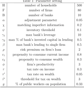
Table 1: Parameter setting
H number of households 500
F number of firms 80
B number of banks 10
α adjustment parameter 0.05
χ matching imperfect information 0.2
ψ inventory threshold 0.1
γ1 max bank’s leverage 10
γ2 max % of bank’s invested capital in lending 0.5
β max bank’s lending to single firm 0.5
ρ risk premium on firm’s loan 2
c1 propensity to consume current income 0.8
c2 propensity to consume wealth 0.3
φ firm’s productivity 3
τ tax rate on income 0.3
τ′ tax rate on wealth 0.05
¯
τ′ threshold for tax on wealth 3
g % of public workers on population 0.33
supply or demand in the credit market and sets an amount of money Mt to reduce the gap
in the following period.
6
Simulations
We run a baseline simulation for a time span ofT =150 periods and analyse the results for the last 50 (so the first 100 are used to initialise the model). Table 1 shows the parameter setting of the baseline simulation. The initial agents’ wealth is set as follows: Af1 =max{0.1, N(3,1)},
Ab1 =max{0.2, N(5,1)}, Ah1 =max{0.01, N(0.5,0.01)}. The policy rate iCBt is constant at
1%.
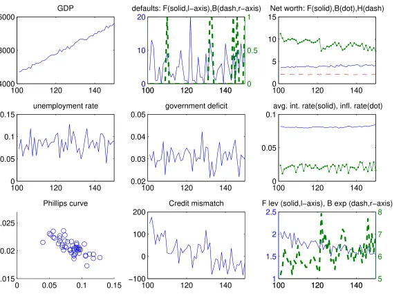
F ig u re 1: B as elin e m o d el: S im u la tio n re su lt s
100 120 140
4000 8000 16000
GDP
100 120 140
0 10 20
defaults: F(solid,l−axis),B(dash,r−axis)
100 120 140 0
0.5 1
100 120 140
0 5 10 15
Net worth: F(solid),B(dot),H(dash)
100 120 140
0 0.05 0.1 0.15
unemployment rate
100 120 140
0.02 0.03 0.04 0.05
government deficit
100 120 140
0 0.05 0.1
avg. int. rate(solid), infl. rate(dot)
0 0.05 0.1 0.15
0.015 0.02 0.025
Phillips curve
100 120 140
−100 0 100 200
Credit mismatch
100 120 140
1 1.5 2 2.5
F lev (solid,l−axis), B exp (dash,r−axis)
100 120 140 5
6 7 8
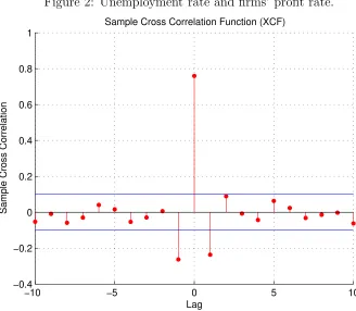
[image:15.842.124.704.76.504.2]correlation at lag 0: the profit rate is high when unemployment is high given that firms save on production costs (e.g., wage bill) but, at the same time, the aggregate demand does not decrease proportionally, because of public workers’ expenditure and consumption due to wealth, thus firms can sell their commodities (including inventories) in the goods market. However, the presence of unemployed people, the tendency of wages to decrease due to the high unemployment rate, and the reduction of households’ wealth, cause the fall of next period aggregate demand that, in turn, reduces firms’ profits. Indeed, Figure 2 displays a negative correlation at lag +1. Instead, the negative correlation at lag -1 means that increasing profits boost the expansion of the economy and then a fall of the unemployment rate follows. The two major innovations we introduce in this agent-based framework, that is (i) the Dynamic Trade-Off theory for firms’ capital structure and its interplay with banks’ credit supply, (ii) the role of an acyclical sector, have opposite effects on business fluctuations. On one hand, firms’ leverage and, in particular, banks’ exposure enlarge business fluctuations: a growing firm requires more credit and, if banks extended new loans, then they are able to expand the production through the employment of more workers; after a while, the rise of employment fosters wages that, together with the rise of interest payments on an increasing debt, reduces firms’ profitability. Thus the business cycle reverses and financial factors amplify the fall of production (the relatively low level of profits with respect to interest payments induces a deleveraging process). In other words, credit is pro-cyclical. In particular, there is a negative but modest correlation between firms’ leverage and the unemployment rate (-0.1539), while there is a more significant negative correlation between banks’ exposure and unemployment (-0.3670). This simulation result is consistent with the empirical evidence on the topic (see, for instance, Kalemli-Ozcan et al., 2011). Accordingly, banks’ capitalization plays a relevant role in determining credit conditions, so influencing firms’ leverage and, in general, the macroeconomic evolution. On the other hand, the presence of an acyclical sector, here represented by the government, has a fundamental role in sustaining the aggregate demand and in mitigating output volatility.
Figure 2: Unemployment rate and firms’ profit rate.
−10 −5 0 5 10
−0.4 −0.2 0 0.2 0.4 0.6 0.8 1
Lag
Sample Cross Correlation
Sample Cross Correlation Function (XCF)
are able to fulfill all credit demand. Accordingly, firms’ mean leverage is influenced by credit availability. The mean interest rate charged by banks on firm loans is 8.11%. Per-capita households wealth (in real terms) is stable around 2.06 (min 2.01, max 2.10), while the same value for firms is equal to 3.91 (min 3.54, max 4.31). Finally, the average ratio between public deficit and GDP is equal to 3.09% (min 2.16%, max 4.22%). It is worth to note that the presence of the government, nevertheless the relatively low level of public deficit, allows for the nominal growth in the model. This outcome also depends on the working of the central bank that finances the government buying public securities charging a low interest rate.
7
Monte Carlo analysis
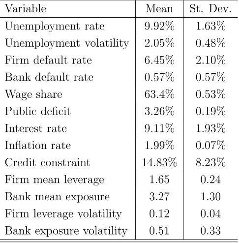
across simulations are: the credit constraint (that is, the fraction of firms’ required credit not fulfilled by banks), and the bank exposure (calculated as the amount of credit lent to firms divided by net worth). The latter variable has a relevant procyclical impact on the economy, that is there is a significant negative correlation between bank exposure and unemployment. In particular, the mean value across simulations is equal to -50.09% (with a standard deviation of 16.03%).
Table 2: Monte Carlo replications: mean values and corresponding standard deviation (calcu-lated over the time span 101-150) of 995 simulations with average unemployment rate below 20%.
Variable Mean St. Dev.
Unemployment rate 9.92% 1.63%
Unemployment volatility 2.05% 0.48%
Firm default rate 6.45% 2.10%
Bank default rate 0.57% 0.57%
Wage share 63.4% 0.53%
Public deficit 3.26% 0.19%
Interest rate 9.11% 1.93%
Inflation rate 1.99% 0.07%
Credit constraint 14.83% 8.23%
Firm mean leverage 1.65 0.24
Bank mean exposure 3.27 1.30
Firm leverage volatility 0.12 0.04 Bank exposure volatility 0.51 0.33
7.1
Financial factors and the real economy
Now we analyse in more detail the relationship between financial variables, like firm leverage and bank exposure, and the unemployment rate (which represents the main real variable in our macroeconomic framework).
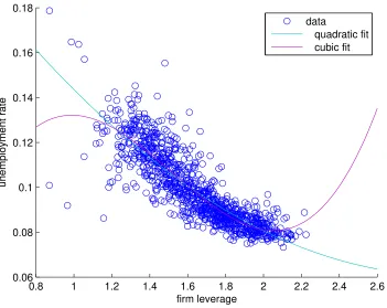
Figure 3 shows that there is a negative non-linear relation between firm leverage and unem-ployment. It is worth to note that for relatively high levels of firm leverage the unemployment rate tends to be smaller and less volatile. However, for largest values of the firm leverage (above 2) the negative relation with the unemployment rate tends to disappear or rather it reverses (as shown by the cubic fit in the Figure).
un-Figure 3: Firm leverage and unemployment rate.
0.8 1 1.2 1.4 1.6 1.8 2 2.2 2.4 2.6
0.06 0.08 0.1 0.12 0.14 0.16 0.18
firm leverage
unemployment rate
data
[image:19.595.115.466.130.409.2]quadratic fit cubic fit
Figure 4: Bank exposure and unemployment rate.
0 1 2 3 4 5 6 7 8
0.06 0.08 0.1 0.12 0.14 0.16 0.18
bank leverage
unemployment rate
data
[image:19.595.114.460.471.746.2]the latter hire more workers and the unemployment rate decreses. But, when the exposure of banks becomes “excessive” this leads to instability (more failures) and an increase of the unemployment rate follows.
7.2
Large crises
In the previous Monte Carlo experiment we observe 5 out of 1000 cases characterised by a large mean unemployment rate (during the period from t = 101 to t = 150). This means that large crises can appear in the macroeconomic system. Moreover, in some simulations we note that the time series of the main macroeconomic variables are non-stationary. In order to check the presence of endogenous regime switches, e.g. from a “normal” period (with average values of variables close to those in Table 2) to a large and extended crisis, we perform an additional Monte Carlo experiment with 100 simulations over a time span of 500 periods (for the same reasons explained above, we discard the first 100 periods of each simulation). In 2 out of 100 simulations the macroeconomic system evolves towards an “extended crisis” scenario, where the private sector tends to disappear, with an unemployment rate above 60%, thus almost only public workers remain employed. In this case, as shown in Figure 5, differently from the usual business cycle mechanism, the decrease of wages due to growing unemployment does not reverse the cycle, but rather amplifies the recession due to the lack of aggregate demand. In other words, the self-adjustment mechanism which spontaneously reverses the business cycle (e.g., the rise of the unemployment rate reduces the real wage and then the resulting increase of profits makes room for an expansionary production phase) does not work. Indeed, real wage lowers excessively boosting a vicious circle for which the fall of purchasing power prevents firms to sell commodities, then firms reduce production, unemployment continues to rise, and the system moves towards a devastating crisis.
In particular, in one of the two extended crises detected in the Monte Carlo experiment, the production system completely crashes and cannot escape this trap without an exogenous intervention. Instead, in the case explained above, the production system does not completely disrupt, then we cannot exclude a recovery in the very long run. But, accordingly to Keynes, “in the long run we are all dead”.
8
Concluding remarks and future research
We present an agent-based macroeconomic model in which heterogeneous agents (households, firms and banks) interact according to a fully decentralized matching mechanism. The match-ing protocol is common to all markets (goods, labor, credit, deposits) and represents a best partner choice in a context of imperfect information.
Figure 5: The extended crisis case: unemployment rate and real wage.
100 150 200 250 300 350 400 450 500
0 0.2 0.4 0.6 0.8
t
unemployment rate (solid line)
100 150 200 250 300 350 400 450 5000.5
1 1.5 2 2.5
real wage (dash−dot line)
of the unemployment rate, the presence of the Phillips curve, the relevance of leverage cycles and credit constraints on economic performance, the presence of bank defaults and the role of financial instability, and the importance of government in providing a fraction of the aggregate demand and then as an acyclical sector which stabilize the economy. In particular, simulations show that endogenous business cycles emerge as a consequence of the interaction between real and financial factors: when firms’ profits are improving, they try to expand the production and, if banks extend the required credit, this results in more employment; the decrease of the unemployment rate leads to the rise of wages that, on the one hand, increases the aggregate demand, while on the other hand reduces firms’ profits, and this may cause the inversion of the business cycle.
“excessive” this leads to instability (more failures) and an increase of the unemployment rate follows. All in all, firm leverage and bank exposure may support the working of the economy (reducing the unemployment rate), but when the levels of both leverage or exposure turn to be excessive, the economy becomes too financially fragile (and unemployment may rise).
Moreover, model simulations highlight that even extended crises can endogenously emerge with a strong reduction of real wages, a consequent fall of the aggregate demand that, in turn, induces firms to decrease production, so enlarging the unemployment rate, in a vicious positive feedback circle. In these cases, the system may remain trapped in a situation, without the possibility to spontaneously recover unless an exogenous intervention.
Our modeling framework can be useful to understand the effects of some policy or institu-tional changes. Indeed, in future developments we will analyse the sensitivity of simulations results to different parameter settings. Moreover, we will also investigate the consequences of alternative assumptions such as the effect of fiscal and monetary policies, labor market rigidity, heterogeneous consumption behavior, etc. Finally, the baseline model presented in this paper will be enriched by adding modules as the interbank market, the stock and bond markets (allowing agents to decide their portfolio allocation), and long-run growth factors (heterogeneous workers’ skills, R&D investments, etc.).
References
[1] Adrian, T., Shin, H.S. (2008) “Liquidity, monetary policy and financial cycles”, Current Issues in Economics and Finance, 14(1), Federal Reserve Bank of New York (Janu-ary/February).
[2] Adrian, T., Shin, H.S. (2009), “Money, Liquidity, and Monetary Policy”, American Eco-nomic Review, 99(2): 600-605.
[3] Adrian, T., Shin, H.S. (2010), “Liquidity and leverage”, Journal of Financial Intermedi-ation, 19(3): 418-437.
[4] Booth L., Asli Demirgu-Kunt V.A., Maksimovic V. (2001), “Capital Structures in De-veloping Countries”, Journal of Finance, 56(1): 87-130.
[5] Brunnermeier M.K., Pedersen L.H. (2009), “Market liquidity and funding liquidity”,
Review of Financial Studies, 22(6): 2201-2238.
[7] Cincotti S., Raberto M., Teglio A. (2012), “Debt Deleveraging and Business Cycles. An Agent-Based Perspective”, Economics - The Open-Access, Open-Assessment E-Journal, Kiel Institute for the World Economy, 6(27).
[8] Dawid H., Neugart M. (2011), “Agent-Based Models for Economic Policy Design”, East-ern Economic Journal, 37(1): 44-50.
[9] Delli Gatti D., Gallegati M., Greenwald B., Russo A., Stiglitz J.E. (2010), “The financial accelerator in an evolving credit network”, Journal of Economic Dynamics and Control, 34(9): 1627-1650.
[10] Diamond D.W., Rajan R. (2000), “A Theory of Bank Capital”, Journal of Finance, 55(6): 2431-2465.
[11] Donaldson G. (1961), “Corporate debt capacity: a study of corporate debt policy and the determination of corporate debt capacity”, Harvard Business School, Harvard University.
[12] Dosi G., Fagiolo G., Roventini A. (2006), “An Evolutionary Model of Endogenous Busi-ness Cycles”, Computational Economics, 27(1): 3-34.
[13] Dosi G., Fagiolo G., Roventini A. (2010), “Schumpeter meeting Keynes: A policy-friendly model of endogenous growth and business cycles”, Journal of Economic Dynamics and Control, 34(9): 1748-1767.
[14] Dosi G., Fagiolo G., Napoletano M., Roventini A. (2012), “Income Distribution, Credit and Fiscal Policies in an Agent-Based Keynesian Model”, LEM Papers Series 2012/03, Laboratory of Economics and Management (LEM), Sant’Anna School of Advanced Stud-ies, Pisa, Italy.
[15] Epstein J.M., Axtell R.L. (1996), Growing Artificial Societies: Social Science from the Bottom Up, MIT Press.
[16] Fagiolo G., Dosi G., Gabriele R. (2004), “Matching, Bargaining, And Wage Setting In An Evolutionary Model Of Labor Market And Output Dynamics”,Advances in Complex Systems, 7(2): 157-186.
[17] Flannery M.J. (1994), “Debt Maturity and the Deadweight Cost of Leverage: Optimally Financing Banking Firms”,American Economic Review, 84(1): 320-31.
[18] Flannery M.J., Rangan K.P. (2006), “Partial adjustment toward target capital struc-tures”,Journal of Financial Economics, 79(3): 469-506.
[20] Frank M.Z., Goyal V.K. (2008), “Tradeoff and Pecking Order Theories of Debt”, in: Espen Eckbo (ed.) The Handbook of Empirical Corporate Finance, Ch. 12: 135-197.
[21] Gaffeo G., Delli Gatti D., Desiderio S., Gallegati M. (2008), “Adaptive Microfoundations for Emergent Macroeconomics”, Eastern Economic Journal, 34(4): 441-463.
[22] Geanakoplos J. (2010), “Leverage cycle”, Cowles foundation Paper No. 1304, Yale Uni-versity.
[23] Godley W., Lavoie M. (2006), Monetary Economics: An Integrated Approach to Credit, Money, Income, Production and Wealth, Palgrave MacMillan.
[24] Graham J.R., Harvey C. (2001), “The Theory and Practice of Corporate Finance”,
Journal of Financial Economics, 60: 187-243.
[25] Greenlaw D., Hatzius J., Kashyap A.K., Shin H.S. (2008), “Leveraged Losses: Lessons from the Mortgage Market Meltdown”,Proceedings of the U.S. Monetary Policy Forum.
[26] Gropp R., Heider F. (2010), “The Determinants of Bank Capital Structure”, Review of Finance, 14(4): 587-622.
[27] He Z., Khang I.G., Krishnamurthy A. (2010), “Balance Sheet Adjustments in the 2008 Crisis”,IMF Economic Review, 58: 118-156.
[28] Hovakimian A., Opler T., Titman S. (2001), “The Debt-Equity Choice”, Journal of Financial and Quantitative Analysis, 36: 1-24.
[29] Jensen M.C., Meckling W.H. (1976), “Theory of the Firm: Managerial Behavior, Agency Costs, and Ownership Structure”, Journal of Financial Economics, 3: 305-360.
[30] Kalemli-Ozcan S., Sorensen B., Yesiltas S. (2011), “Leverage Across Firms, Banks, and Countries”, NBER Working Papers 17354.
[31] Kinsella S., Greiff M., Nell E. (2011), “Income Distribution in a Stock-Flow Consistent Model with Education and Technological Change”, Eastern Economic Journal, 37(1): 134-149.
[32] LeBaron B., Tesfatsion L.S. (2008), “Modeling Macroeconomies as Open-Ended Dynamic Systems of Interacting Agents”, American Economic Review, 98(2): 246-250.
[33] Lemmon M., Roberts M., Zender J. (2008), “Back to the beginning: Persistence and the cross-section of corporate capital structure”,Journal of Finance, 63: 1575-1608.
[35] Myers, S.C. (1977), “Determinants of corporate borrowing”, Journal of Financial Eco-nomics, 5(2): 147-175
[36] Myers S.C., Majluf N.S. (1984), “Corporate Financing and Investment Decisions When Firms Have Information that Investors Do Not Have”, Journal of Financial Economics, 13: 87-224.
[37] Rajan R., Zingales L. (1995), “What do we know about capital structure? Some evidence from international data”, Journal of Finance, 50: 1421-1460.
[38] Riccetti L., Russo A., Gallegati M. (2011), “Leveraged Network-Based Financial Ac-celerator”, Quaderno di Ricerca 371, Department of Economics and Social Sciences, Universit`a Politecnica delle Marche.
[39] Russo A., Catalano M., Gaffeo E., Gallegati M., Napoletano M. (2007), “Industrial dynamics, fiscal policy and R&D: Evidence from a computational experiment”, Journal of Economic Behavior & Organization, 64(3-4): 426-447.
[40] Seppecher P. (2012), “Flexibility of wages and macroeconomic instability in an agent-based computational model with endogenous money”,Macroeconomic Dynamics, 16(s2): 284-297.