Munich Personal RePEc Archive
Reference dependent ambiguity aversion:
theory and experiment
Qiu, Jianying and Weitzel, Utz
Radboud University Nijmegen, Department of Economics,
Nijmegen, the Netherlands
1 November 2011
Online at
https://mpra.ub.uni-muenchen.de/35289/
Reference Dependent Ambiguity Aversion: Theory and
Experiment
Jianying Qiu∗ Utz Weitzel†
December 8, 2011
Abstract
In standard models of ambiguity, the evaluation of an ambiguous asset, as of a risky asset, is considered as an independent process. In this process only information directly pertaining to the ambiguous asset is used. These models face significant challenges from the finding that ambiguity aversion is more pronounced when an ambiguous asset is evaluated alongside a risky asset than in isolation. To explain this phenomenon, we developed a theoretical model based on reference dependence in probabilities. According to this model, individuals (1) form subjective beliefs on the potential winning probability of the ambiguous asset; (2) use the winning probability of the (simultaneously presented) risky asset as a reference point to evaluate the potential winning probabilities of the ambiguous asset; (3) code potential winning probabilities of the ambiguous asset that are greater than the reference point as gains and those that are smaller than the reference point as losses; (4) weight losses in probability heavier than gains in probability. We tested the crucial assumption, reference dependence in probabilities, in an experiment and found supporting evidence.
Keywords: Ambiguity Aversion, Reference Point, Comparison, Experiment
JEL classification: C91, D03, D81
∗Department of Economics, Radboud University Nijmegen, Thomas van Aquinostraat 5.12, 6525 GD
Nijmegen, the Netherlands, Email: [email protected]
†Department of Economics, Radboud University Nijmegen, Thomas van Aquinostraat 5.12, 6525 GD
1
Introduction
The evaluation of ambiguous assets is much more complicated than risky assets due to
the absence of objective probabilities. Savage (1972) suggests that individuals could form
subjective additive beliefs. The subjective beliefs could then be used to evaluate the
ambiguous assets according to the expected utility theory. Ellsberg (1961), however,
presented compelling examples in which people prefer to bet on known rather than on
unknown probabilities. One version of the Ellsberg paradox is as follows: There are two
urns: a known urn and an unknown urn. The known urn contains 50 white and 50 black
balls. The unknown urn also contains 100 black and white balls, but the proportion of
black and white balls is unknown. For either urn, an individual first chooses a color and
then draws a ball from the urn. She receives 100 if the color of chosen ball matches her
chosen color. Typically, an individual is willing to pay less for the gamble on the unknown
urn than on the known urn. Several variations of Ellsberg’s (1961) original designs have
been implemented in laboratory experiments, and a similar discount on the unknown
urn was observed (see Camerer and Weber, 1992, for a review of the literature). This
phenomenon, termed ambiguity aversion, is inconsistent with Savage’s (1972) subjective
expected utility model.
Ambiguity aversion has received tremendous research interest and numerous models have
been put forward to explain it: Schmeidler’s (1989) Choquet expected utility, Gilboa
and Schmeidler’s (1989) maxmin expected utility, Klibanoff et al.’s (2005) smooth
am-biguity model; Nau’s (2006) multistage recursive model, and Abdellaoui et al.’s (2011)
non-expected utility model of source functions, to name just a few leading examples.
These approaches face serious descriptive difficulties since the work of Fox and Tversky
(1995). They showed that the willingness to pay for the ambiguous asset was not
system-atically different from the risky asset when each of them was evaluated in isolation. Only
when the ambiguous asset was evaluated alongside the risky asset, ambiguity aversion
became more pronounced. Fox and Tversky (1995) refer to this effect as ‘comparative
ig-norance’. Chow and Sarin (2002) and Fox and Weber (2002) extended Fox and Tversky’s
aversion results from the fact that the ambiguous and the risky asset were evaluated
to-gether. This is a fundamentally different perspective of the evaluation of an ambiguous
asset. As stated by Wakker (2000): “Fox and Tversky’s finding seems to place the Ellsberg
paradox in an entirely new light”.
In standard models of ambiguity, the evaluation of an ambiguous asset, as of a risky
as-set, is considered to be an independent process. In this process only information directly
pertaining to the ambiguous asset is used. We believe, while this assumption seems
appro-priate for the evaluation of a risky asset with clearly defined objective probabilities, it is
too strong for the evaluation of an ambiguous asset. Given that there is little information
about the ambiguous asset per se, it seems natural that individuals attempt to ‘improve’
their evaluation of the ambiguous asset by using other information. One reasonable way
would be to find a risky asset with a similar structure and use it as reference. As a result,
the evaluation of the ambiguous asset becomes simpler and clearer. We therefore suggest
that individuals are inclined to use of the information pertaining to the risky asset in the
evaluation of the ambiguous asset when the two types of assets are presented together.
Empirical studies on ambiguity aversion typically used the same monetary payoff structure
between the risky asset and the ambiguous asset. Also, in almost all valuation models of
ambiguous assets payoffs and probabilities are treated separately. Thus, with the same
payoff structure, the manipulation of probabilities seems to remain as the only explanation
for Fox and Tversky’s (1995) findings without introducing additional effects. Based on
this observation, we hypothesize that, when the risky asset and the ambiguous asset
are presented together, (1) individuals form subjective beliefs on the potential winning
probability of the ambiguous asset; (2) they use the winning probability of the risky asset
as the reference point to evaluate the potential winning probabilities of the ambiguous
asset; (3) analogous to prospect theory where payoffs are coded as gains or losses relative
to a reference point, they code potential winning probabilities of the ambiguous asset that
are greater than the reference point as gains and probabilities smaller than the reference
point as losses; (4) finally and again in analogy to prospect theory, individuals exhibit
loss aversion in probability by assigning a larger weight to losses in probability than to
as ‘reference-dependence hypothesis’. Further, in order to distinguish between ambiguity
aversion in isolation and ambiguity aversion in combination with a risky asset, we shall
call the latter ‘reference-dependent ambiguity aversion’.
Our approach differs substantially from the prevailing explanation of comparative
igno-rance, which is typically interpreted as a companion of the “competence hypothesis”
(Heath and Tversky, 1991). According to this hypothesis, people try to avoid
ambigu-ity in areas of incompetence, while they exhibit less ambiguambigu-ity aversion if they feel more
competent in the decision domain. Referring to the competence hypothesis, Fox and
Tversky (1995) and Heath and Tversky (1991) argue that the joint presentation of the
two assets highlights the relative incompetence about the ambiguous urn, resulting in a
lower value for it.
The aim of this paper is to accommodate Fox and Tversky’s (1995) findings without
in-troducing additional elements such as individuals’ perceptions of competence. The central
idea of our approach is the use of the risky asset as a reference point in probability for the
evaluation of the ambiguous asset. In doing this, we are more in line with (cumulative)
prospect theory and not the competence hypothesis. We tested our crucial assumption,
the reference-dependence of ambiguity aversion, in an experiment and found supporting
evidence.
In many studies, ambiguity aversion is also found without an explicit comparable risky
asset. Chow and Sarin (2002), for example, while finding evidence consistent with Fox
and Tversky (1995), also report sizable ambiguity aversion without a directly comparable
risky asset. This finding is not inconsistent with our model. Even when the ambiguous
asset is valued in isolation, individuals might still try to simplify the evaluation process by
finding a reference that is not explicitly presented. Such a reference is often rather salient.
For example, in the two-color Ellsberg urn mentioned above it seems natural to think of
the probability 0.5 as the reference. Fox and Weber’s (2002) study on, inter alia, order
effects also indicates that reference-dependent ambiguity aversion can extend beyond a
directly comparative evaluation context. Of course, individuals might be less loss averse
The paper proceeds as follows. Section 2 demonstrates the theoretical model, Section 3
presents the experimental design. Results are reported in Section 4. Finally, Section 5
concludes.
2
The Model
There are two assets, one is risky (denoted by R) and the other is ambiguous (denoted
by U). To simplify the derivation, let’s assume that there are only two states of world:
a good state and a bad state. For the risky asset there is an objective probability p0 for
the good state (and thus 1−p0 for the bad state). Individuals receive some monetary
payment Gif the good state realizes, and zero otherwise. We let v(G) denote the utility
or value that individuals attach to a monetary payoff ofG, where v(0) = 0. Without loss
of generality, we normalize v(G) ≡ 1. Since our main purpose is a descriptive one, we
followed prospect theory (Kahneman and Tversky, 1979; Tversky and Kahneman, 1992).
We assume that individuals evaluate the risky asset in the following way:
V(R) =π(p0)v(G) =π(p0), (1)
whereπ(p0) is the probability weighting function.
For the ambiguous asset, there is no clear probability one can assign to the good state.
One can, however, form a subjective belief for the good state. Letpdenote the subjective
probability an individual assigns to the good state, and let F(p) denote the cumulative
subjective belief distribution that the individual has about the probabilityp. Then, if an
individual behaves according to the subjective expected utility model, she should evaluate
the ambiguous asset as follows:
V(U) =v(G)
Z 1
0
pdF(p), (2)
which is independent ofp0 (and therefore the value of the risky asset).
to evaluate her subjective probability of the good state under ambiguity. Analogous to
prospect theory, where payoffs are coded as gains or losses relative to a reference point,
we assume that the individual codesplarger thanp0 as gains in probability andpsmaller
than p0 as losses in probability. Moreover, the individual evaluates gains and losses in
probability differently. Let l(p−p0), p < p0, denote the way the individual evaluates
losses in probability, andg(p−p0),p≥p0 denote the way the individual evaluates gains
in probability. Let ∆ denote the absolute difference betweenpandp0. In the spirit of loss
aversion in prospect theory, we assume that−l(−∆)> g(∆),∀∆∈[0,1], i.e. for any equal
amount of difference in probability losses in probability are always weighted more heavily
than gains in probability. With above assumptions, the evaluation process becomes
V(U) =π(p0) +
ambiguity component
z }| {
Z p0
0
l(p−p0)dF(p) +
Z 1
p0
g(p−p0)dF(p). (3)
In equation (3) there are essentially two components. The first component captures an
individual’s evaluation of the risky asset within the framework of prospect theory. The
second component, the sum of the two integrals, captures an individual’s evaluation of
the ambiguous asset. We refer to the latter as “ambiguity component”. When the
am-biguity component is zero, individuals are amam-biguity neutral, because their values for the
ambiguous and for the risky asset are the same. This would happen when individuals
have a degenerated point belief at p0. When the ambiguity component is negative, the
ambiguous asset is valued lower than the comparable risky asset and there is
ambigu-ity aversion. When the ambiguambigu-ity component is positive, the ambiguous asset would be
evaluated higher than the risky asset and individuals are ambiguity seeking.
In our model the subjective perception of the levels of ambiguity and individuals’ attitudes
toward ambiguity are separated from each other. The former is captured by the subjective
beliefsF(p). The higher the standard deviation ofF(p), the more ambiguous the individual
perceives the situation. The maximum ambiguity is obtained when F(p) is uniformly
distributed between 0 and 1. The latter is captured by the functionsl(−∆) andg(∆).
here and the probability weighting functions used in (cumulative) prospect theory
(Kah-neman and Tversky, 1979; Tversky and Kah(Kah-neman, 1992) must be made. In (cumulative)
prospect theory, π+ (π−) stands for the probability weighting function for gains (losses)
in the payoff domain. Although the two probability weighting functions are allowed to
be different in gains and losses of payoffs, this difference is not important for any of the
central results in prospect theory. Also, empirically there is no strong evidence suggesting
differences between the two functions. The g(∆) and l(−∆) we used here represent the
evaluation functions of gains and of losses in the probability domain. We assume that
individuals weight losses in probability heavier than gains in probability. This assumption
is the main driving force of our model. In prospect theory a closer companion tog(∆) or
l(−∆) would be the value functions of payoffs in gains or losses.
Apart from this assumption, the parametric form of the two functions can be rather
general. It is not even required that the two functions are continuous or differentiable.
Yet, it could be useful to think of some simple and intuitive ways of capturing loss aversion
in probability. Analogous to the definition of loss aversion in prospect theory we could
choose the following specification: g(∆) = ∆α and l(−∆) =−λ(∆)α, where λ > 1 is the loss aversion coefficient andαis some constant. Another specification could beg(∆) = ∆α
andl(−∆) =−(∆)β, whereα > βcaptures loss aversion in probability. Since our theory is
mainly motivated by loss aversion in prospect theory, we shall use the former to illustrate
the main features of the model. Using the latter does not change the result qualitatively.
2.1 Some Examples
In the following we will use a few examples to provide an intuitive illustration of the
implications of the ambiguity component in equation (3). Let’s assume that the subjective
belief of p is uniformly distributed between 0 and 1, i.e. F(p) = p. This assumption is
strictly for illustrative purposes. In general, F(p) should be context specific and could
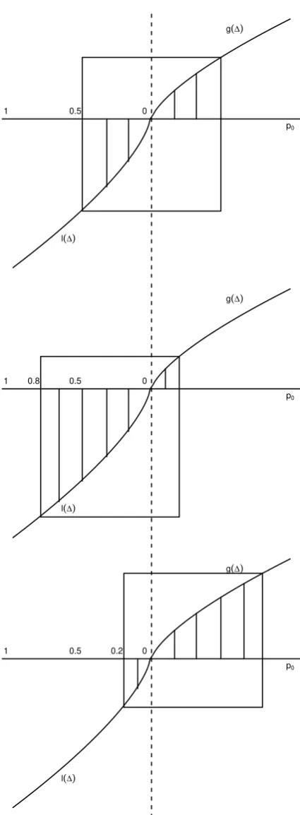
be different for different individuals. Figure 1 illustrates the calculation of the ambiguity
component. Notice first that, when F(p) = p, the integral Rp0
0 l(p−p0)dF(p) simply
area below the lineg(∆).
Consider first the Ellsberg paradox, where the objective probability of the risky asset is
0.5. In this case, p0 = 0.5, and thus the ambiguity component is
Ambiguity component =
Z 0.5
0
l(p−0.5)dF(p) +
Z 1
0.5
g(p−0.5)dF(p). (4)
This is illustrated in the top graph of Figure 1. Since−l(−∆)> g(∆),∀∆∈[0,1] , it can
be immediately seen that the negative area (bottom left) is larger than the positive area
(top right). Hence, the ambiguity component is negative,
Ambiguity component =
Z 0.5
0
l(p−0.5)dF(p) +
Z 1
0.5
g(p−0.5)dF(p)
< −
Z 1
0.5
g(p−0.5)dF(p) +
Z 1
0.5
g(p−0.5)dF(p) = 0, (5)
which represents ambiguity aversion in the Ellsberg paradox. Note that this result can
be obtained for anyF(p) that gives a symmetric density mass around p0, as long as the
assumption of loss aversion in probability is satisfied.
In some ambiguous situations we could havep0 larger than 0.5. For example, let’s consider
two urns, each with 100 balls of five colors: black, white, yellow, green, and blue. In the
risky urn there are 20 balls for each color. In the ambiguous urn the proportion of colored
balls is unknown. For each urn, an individual can choose four colors and wins if the
drawn ball matches any of the four colors. In this scenario, p0 = 0.8, and the ambiguity
component is:1
Ambiguity component =
Z 0.8
0
l(p−0.8)dF(p) +
Z 1
0.8
g(p−0.8)dF(p). (6)
The calculation is illustrated in the middle graph of Figure 1. As the negative area is larger
1
In this scenario the assumption of F(p) = p is questionable. As discussed later, a more natural assumption ofF(p) would perhaps be a distribution which assigns density mass symmetric top0 = 0.8. In
1 0.5 0
p0
l(∆)
g(∆)
1 0.8 0.5 0
p0
l(∆)
g(∆)
1 0.5 0.2 0
p0
l(∆)
[image:10.595.194.407.85.663.2]g(∆)
Figure 1: The graph is produced by assuming F(p) = p, g(∆) = ∆0.7, and l(∆) =
than the positive area, the ambiguity component is negative and, consequently, there is
ambiguity aversion.
Finally, in some ambiguous situations we could havep0 much smaller than 0.5. Consider
the two five-color-urns mentioned above. For each urn, an individual can now choose only
one color and wins if the drawn ball matches this color. In this scenario, p0 = 0.2, and
the ambiguity component is:
Ambiguity component =
Z 0.2
0
l(p−0.2)dF(p) +
Z 1
0.2
g(p−0.2)dF(p). (7)
As illustrated in the bottom graph of Figure 1, the negative area is now smaller than the
positive area, and, consequently, the ambiguity component is positive. That is, in
situa-tions where the objective reference probability is small, individuals are ambiguity seeking.
This result is not as unusual as it may first appear. In fact, several studies provided
evidence of ambiguity seeking when the objective probability of winning an ambiguous
gamble was small (see Camerer and Weber, 1992, Table 3, for an overview).
2.2 Links to Other Models
So far, purely for illustrative purposes, we have assumed F(p) = p when p0 is small
(p0 = 0.2), medium (p0 = 0.5), and large (p0 = 0.8). This is, of course, an ad hoc
assumption, which becomes questionable whenp0moves away from 0.5. An arguably more
reasonable assumption ofF(p) would be thatF(p) exhibits more mass aroundp0, and the
furtherpmoves away fromp0, the less mass individuals attach to these probabilities. One
such form of subjective belief, for example, is a normal distribution with a mean p0 and
values that are restricted to [−p0,1−p0].2
2
Since the normal distribution has values extending outside of the range [−p0,1−p0], the restriction
ofp∈[−p0,1−p0] makes the cumulative mass in the range of [−p0,1−p0] smaller than 1. For a proper
distribution function, one could adjust the normal distribution function to
1 N(−p0,1−p0)
×dN(p),
0.0 0.2 0.4 0.6 0.8 1.0
0.0
0.2
0.4
0.6
0.8
1.0
p0
w
eights
π(p0)=e(−0.93(−ln(p0))
0.85)
[image:12.595.133.455.123.414.2]Π(p0)
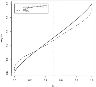
Figure 2: The parametric form of π(p0) = e−0.93(−ln(p0))
0
.85
is taken from the empirical estimate of Abdellaoui et al. (2011). The functional form of Π(p0) is produced by assuming
g(∆) = ∆ and l(−∆) = −1.5∆. F(p) is assumed to be normally distributed around p0
with a standard deviation of 0.20.
As we normalized V(G) ≡ 1, the value of the risky asset is simply π(p0). We can take
a similar perspective for the value of the ambiguous asset. LetV(U) ≡Π(p0), we could
regard the value of the ambiguous asset as its weighting function in an ambiguous
situa-tion. A comparison betweenπ(p0) and Π(p0) then reflects the difference between decision
making under risk and under ambiguity. Figure 2 provides such a comparison.
Figure 2 bears a remarkable similarity to Figure 3 in Abdellaoui et al. (2011). In particular,
our theory suggests, similar to their empirical findings, that: (1) individuals are ambiguity
seeking with smallp0and ambiguity averse with largep0; (2) decision weights in ambiguity,
in probability under ambiguity than under risk. Note that Abdellaoui et al.’s (2011) results
were obtained without explicit comparison between the ambiguous and the risky asset.3
However, in their experimental setting, there often exists a salient probability that may
be used as reference.4 Hence, although the subjects in Abdellaoui et al.’s (2011) study did
not explicitly face a risky asset as comparison, they might nevertheless have formed an
implicit reference when evaluating the ambiguous asset. Of course, based on the finding
of Fox and Tversky (1995), ambiguity aversion should be weaker when the reference is
not explicit. This may explain why our model suggests a stronger certainty effect than
the empirical findings in Abdellaoui et al. (2011), as revealed by a larger gap in our curve
whenp0 approaches 0 or 1.5
3
Experimental Design
The crucial assumption in our model is the reference-dependence hypothesis, which states
that the objective probability of the risky asset is used as a reference to evaluate the
subjective probability of the underlying state of the ambiguous asset. Thus, unlike other
models of ambiguity, our model suggests that the probability of the risky asset has an
impact on the value of the ambiguous asset.
We decided to directly employ a relatively strong test condition: we held the ambiguous
asset constant while we varied the winning probabilities of the risky asset. As the
am-biguous asset remains the same, its value should, according to standard ambiguity models,
remain constant no matter what risky asset is presented with it. If, however, the value
of the ambiguous gamble changes with the variations in the probabilities of the risky
as-3
Abdellaoui et al. (2011) used the certainty equivalence method to obtain the value of the ambiguous asset and the risky asset, but they never presented the two assets simultaneously to subjects.
4
For example, for the two five-color-urns (with 100 balls) mentioned earlier, it seems reasonable to assume thatp0 = 0.2 andp0 = 0.8 are the most prominent comparable probabilities in the minds of the
subjects, even if they are not displayed simultaneously when they take their decisions.
5
The shape of Π(p0) certainly depends on the assumption ofF(p) and the particular parametric forms
ofl(−∆) andg(∆). The general properties of Π(p) are rather robust. We simulated Π(p0) with a few
set, this direct effect can be interpreted as strong support for the reference-dependence
hypothesis.
Another, more elaborate way of testing the our model is to vary the winning probabilities of
the risky assets alongside several values of fixed underlying probabilities of the ambiguous
asset. The willingness to pay (WTP) for the risky and for the ambiguous asset could then
be used to produce a graph similar to the one in Figure 2. However, as this test would
primarily focus on the extended model, it is unnecessarily complicated for a basic test of
the reference-dependence hypothesis.
Given that the ambiguous asset is fixed, a between-subjects design becomes a natural
choice. We administered to each subject a questionnaire that described two gambles: one
ambiguous and one risky. The ambiguous gamble was presented as a bag with 10 black
and white chips of unknown proportion. The subject could first choose a color (white or
black) and then draw a chip out of the bag. If the color of the chip matched the chosen
color, she won 10 euro, and zero otherwise.6 Similarly, the risky gamble was presented as
a bag with 10 black and white chips of known proportion. The subject drew a chip out of
the bag and if the chip was black, she won 10 euro, and zero otherwise. An example of the
the questionnaire is shown in Figure 4 and Figure 5 in the Appendix. In all questionnaires,
the ambiguous gamble was held constant and thus all subjects faced the same ambiguous
gamble. Different subjects, however, faced different risky gambles. There were seven risky
gambles: a bag withnblack chips of a total 10 chips, wheren=1, 3, 4, 5, 6, 7, or 9. These
seven bags corresponded to seven risky gambles with a winning probability of 0.1, 0.3, 0.4,
0.5, 0.6, 0.7, or 0.9 respectively, constituting seven treatments.
Individuals typically read questionnaires from the left to the right. If individuals evaluate
the gamble on the left hand side first, they might be more inclined to use the probability
of the risky asset as the reference when it is presented on the left hand side. To test for
such an order effect, we counter balanced the sides on which the risky and the ambiguous
6
gamble were presented.
We elicited subjects’ WTP for the risky gamble and the ambiguous gamble by using the
BDM mechanism (Becker et al., 1964). For the real payment of a subject, we generated
a random number between 0 and 10 (by drawing a chip from a bag with 11 respectively
numbered chips). The drawn number would then be compared with her WTP for the
gamble on either the left or the right hand side (determined by a coin flip) of the
ques-tionnaire. If her WTP was smaller than the randomly generated number, then she would
not get to play the gamble and her experiment ended. If the subject’s WTP was equal
to or larger than the randomly generated number, then she played the gamble, but payed
only the price of the randomly generated number.
Constructing the ambiguous gamble properly is critical to the experiment. Although the
construction procedure must be perfectly clear, the gamble itself should be regarded by
students as ambiguous. We constructed the ambiguous gamble according to the following
procedure, which was announced publicly before we implemented it. At the start of the
experiment we asked ten randomly selected subjects, who did not participate in rest of
the experiment, to pick an integer number between 0 to 10. We did not tell them how
are we going to use those numbers. Each of them left the experimental room, secretely
wrote the number on a small piece of paper, which they then folded, to hide the number.
They then brought the folded pieces of paper into the experimental room and we asked
another randomly chosen subject, who did not participate in rest of the experiment, to
help us with the construction of the ambiguous gamble. This helper randomly picked one
of the ten folded papers. We then gave the helper two bags: one with 10 black chips and
one with 10 white chips. We asked the helper to leave the experimental room and use the
two bags to produce an ambiguous bag of 10 chips, in which the number of black chips
should be the number on the paper she has drawn. When finished, the helper returned
with two closed bags, placed the ambiguous bag on the desk in the front and stashed the
other away. Neither the experimenters nor the subjects knew the contents of any of the
two bags throughout the experiment.
The subjects were 210 second year business and economics students in the bachelor course
“Corporate Finance” (third lecture). Before the lecture started, we placed the
question-naires on the desks, with the back side facing up. To reduce the influence of peer students
on one’s decisions, we always left one empty seat between any two seats. Furthermore, we
distributed the questionnaire in such a way that every student was surrounded by
differ-ent treatmdiffer-ents. When the lecture started, we guided studdiffer-ents to their seats in an orderly
manner. We asked them not to touch the questionnaire on the desk until we told them so.
They were also told that they could read the side that was facing up (which explained the
payment procedure). Once the classroom was filled, we did not allow the rest of students
to enter the classroom. They waited outside the classroom where we gave them some
questionnaires to fill in to avoid making them feel excluded. Those questionnaires are,
however, excluded from data analysis. After all students were seated, we asked them to
flip the questionnaire around and to read the front side of questionnaire, but not to fill
in the questionnaire yet. We gave students five minutes to read questionnaires. After the
five minutes, we asked students to once again turn to the back side of the questionnaire.
We then read through the payment procedure aloud. We told the students that 20 of
them would be chosen for real payment after the lecture. Subjects that were chosen for
real payment would receive an endowment of 10 euro. In our explanations of the payment
procedure, special attention was given to the BDM mechanism.7 We asked students to
raise their hands if they had any questions. Questions were answered individually.
We then carefully explained the procedure of constructing the ambiguous gamble (as
described above). After the ambiguous gamble was produced, we placed the ambiguous
bag on a desk in front of all students. We told them explicitly that this was the ambiguous
bag described in their questionnaires. Questionnaires were then filled in and collected.
Each student retained an ID number that was also printed on the questionnaire. Then
the lecture started. In a 15-minute break, after the first half of the lecture, we asked the
student helper to randomly pick 20 questionnaires out of the pile. The ID numbers of
these questionnaires were announced and shown on a screen. The students with these ID
7
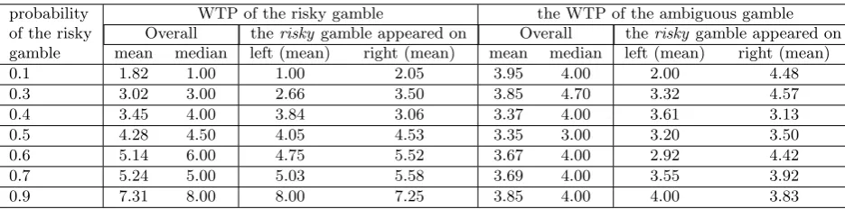
probability WTP of the risky gamble the WTP of the ambiguous gamble of the risky Overall theriskygamble appeared on Overall therisky gamble appeared on gamble mean median left (mean) right (mean) mean median left (mean) right (mean) 0.1 1.82 1.00 1.00 2.05 3.95 4.00 2.00 4.48 0.3 3.02 3.00 2.66 3.50 3.85 4.70 3.32 4.57 0.4 3.45 4.00 3.84 3.06 3.37 4.00 3.61 3.13 0.5 4.28 4.50 4.05 4.53 3.35 3.00 3.20 3.50 0.6 5.14 6.00 4.75 5.52 3.67 4.00 2.92 4.42 0.7 5.24 5.00 5.03 5.58 3.69 4.00 3.55 3.92 0.9 7.31 8.00 8.00 7.25 3.85 4.00 4.00 3.83
Table 1: WTPs of the risky gamble and the ambiguous gamble. “Left” (“right”) means the risky gamble was on the left (right) hand side of the questionnaire.
numbers were asked to stay after the lecture. The rest was allowed to also stay and watch
the experiment, but they needed to be quiet. After the lecture was over, we asked the
20 students to come to the front of the classroom and show their ID number. For each
student, we then determined via the BDM mechanism whether they could really play the
gamble, as described above. Those who could not play the gamble received 10 euro and
stayed outside of the experimental area. The others played the gamble.8
In total the experiment (exluding lecture time) lasted about 45 minutes and the average
payoff of the selected students was 9.88 Euro.
4
Experimental results
In total 210 students participated the experiment. Two students did not give their WTPs
for the ambiguous gamble, and were therefore excluded from analysis.
Table 1 summarizes the WTPs of the risk gambles with 1, 3, 4, 5, 6, 7, 9 black chips
(corresponding a winning probability of 0.1, 0.3, 0.4, 0.5, 0.6, 0.7, 0.9), and WTPs of
the ambiguous gamble that were presented along with them. We further split the WTPs
by the positioning of the risky gamble on the questionnaire, that is, whether the risky
gamble was shown on the left or on the right side of the questionnaire. As can be seen by
8
comparing the WTPs of the ambiguous and the risky gamble on the row of 0.5 winning
probability, there is significant ambiguity aversion. The mean and median WTPs of the
risky gamble with 0.5 winning probability are 4.28 and 4.5, whereas the mean and median
of the ambiguous gamble are 3.35 and 3.0, respectively. A two-sided wilcoxon test shows
that the difference is significant (p <0.01).
If students behaved according to standard models of ambiguity, we should not observe
much variation of the WTPs of the ambiguous gamble when the probability of the risky
gamble changes. This is clearly not what we observed in the data. As we can see from
Table 1, the ambiguity aversion is most pronounced when the risky gamble has a winning
probability of 0.5: the mean difference of WTPs between the risky and the ambiguous
gamble is 0.93 and the median difference is 1.5. The WTPs of the ambiguous gamble
increases (hence ambiguity aversion, defined as the difference of WTPs between the risky
gamble withp0 = 0.5 and the ambiguous gamble, decreases) as the winning probability of
the risky gamble moves away fromp0 = 0.5: mean differences of ambiguity aversion are
0.91, 0.43, and 0.33 respectively for the risky gamble with winning probability of 0.4, 0.3,
and 0.1, and are 0.61, 0.59, 0.43 respectively for the risky gamble with winning probability
of 0.6, 0.7, and 0.9; median difference of−0.2 for the risky gamble with winning probability
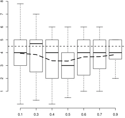
of 0.3 and median difference of 0.5 for others. An graphic illustration is reported in Figure
3.9 In this graph, the x-axis is the winning probability of the risky gambles: p
0=0.1, 0.3,
0.4, 0.5, 0.6, 0.7, 0.9, the y-axis is a boxplot of the values of the ambiguous gamble. The
difference between the WTPs of the ambiguous gamble atp0= 0.5 and all other values of
p0 is statistically significant at a 90 percent confidence interval (two-sided Wilcoxon test,
p= 0.0802). We also tested the difference between the WTPs of the ambiguous gamble at
p0= 0.5 and (jointly) at p0 = 0.1 and 0.3, and betweenp0 = 0.5 and (jointly) atp0 = 0.7
and 0.9. Again, both differences are significant at a 90 percent confidence interval
(two-sided wilcoxon tests, p = 0.0595 and p = 0.0925, respectively). Among the ambiguous
gambles with p0 6= 0.5 there is no single pair with statistically significant differences in
their WTPs (two-sided wilcoxon tests,p >0.1 for each pair).
9
One should not compare this figure with Figure 2. Figure 2 is produced by varying the ambiguous gamble along withp0, in such a way that the ambiguous gamble has an “ambiguity neutral” probability
0.1 0.3 0.4 0.5 0.6 0.7 0.9
1
2
3
4
5
6
7
[image:19.595.190.409.255.460.2]8
The students typically read from the left to the right. This implies that they could have
read and evaluated the left hand side gamble first. This could have an important
implica-tion for our model: if the risky gamble was posiimplica-tioned on the left hand side, subjects might
have been more inclined to use its winning probability as reference for the ambiguous
gam-ble on the right hand side than the other way around. Consequently, reference-dependent
ambiguity aversion could be more pronounced when the risky gamble was shown on the
left hand side. To check this possibility we compared the WTPs of the ambiguous gamble
when the risky gamble was presented on the left and on the right. We find statistically
significant differences in WTPs for ambiguous gambles that were presented with the risky
gambles of 0.1, 0.3, and 0.6 winning probabilities (one-sided wilcoxon test, p <0.05). In
contrast, when the risky gambles of 0.4 and 0.9 were on the left hand side the average
am-biguous WTPs were even lower, although not statistically significant (two-sided wilcoxon
test, p > 0.10). All together, there seems to be a tendency for a more pronounced
am-biguity aversion on the right hand side of the questionnaire, but the evidence is sparse.10
This result is consistent with the finding in Alevy (2011), where they found that subjects
priced ambiguous assets lower than risky assets only when they were previously exposed
to risky assets.
We calculated each subject’s risk aversion as the difference of the risk neutral evaluation
10×p and her WTP for the risky gamble. As a measure of ambiguity aversion, we
subtracted each subject’s WTP for the ambiguous gamble from the mean of the risky
gamble with a winning probability of 0.5 (4.28 on average). We then computed the
non-parametric Spearman correlation of the risk aversion and ambiguity aversion and found
a statistically significant positive correlation of 0.49 (p < 0.01). This result is consistent
with the study of Bossaerts et al. (2010), where the authors suggest that a positive
risk-ambiguity correlation may be able to explain the ‘value effect’ in historical financial market
data.
10
5
Discussion
In this paper we propose a novel approach to explain ambiguity aversion. The central
idea is the use of a more or less salient reference point in probability for the evaluation of
the ambiguous asset. We argue that individuals form subjective beliefs on the potential
winning probability of the ambiguous asset and that the winning probability of risky asset
in the classic setting of Fox and Tversky (1995) is used as a reference point to evaluate
the potential winning probabilities of the ambiguous asset. Analogous to prospect theory
where payoffs are coded as gains or losses relative to a reference point, potential winning
probabilities of the ambiguous asset that are greater than the reference point are coded as
gains and probabilities smaller than the reference point are coded as losses, and individuals
exhibit loss aversion in probability by assigning a larger weight to losses in probability than
to the same amount of gains in probability. We tested the crucial assumption of the model,
reference-dependence, in an experiment and found supporting evidence.
Our approach and explanation of ambiguity aversion is fundamentally different from
stan-dard models, which attempt to explain ambiguity aversion as an isolated phenomenon.
Also, our approach differs from the predominant explanation of comparative ignorance,
first presented by Fox and Tversky (1995). As a companion of the competence hypothesis
(Heath and Tversky, 1991), the comparative ignorance hypothesis per se does not depend
on a comparison or even a reference point, but on the perception of (in)competence as
a state of mind. Although the original experimental design presentated the risky and
the ambiguous urn together, (in)competence about an ambiguous situation can also be
created in settings without direct comparisons where the ambiguous urn is effectively
eval-uated in isolation (see e.g. Camerer and Weber, 1992), but under different perceptions of
competence.
In contrast, our approach does not assume that ambiguity is evaluated in isolation. We
suggest that people try to evaluate ambiguity by comparing it to a similar, but less
am-biguous situation of, ideally, pure risk. If such a salient risky comparison exists, we argue
References
Abdellaoui, M., Baillon, A., Placido, L., and Wakker, P. P. (2011). The rich domain
of uncertainty: Source functions and their experimental implementation. American
Economic Review, 101(2):695–723.
Alevy, J. E. (2011). Ambiguity in individual choice and market environments: On the
importance of comparative ignorance. Technical report.
Becker, G., DeGroot, M., and Marschak, J. (1964). Measuring utility by a single-response
sequential method. Behavioral Science, 9(3):226–232.
Bossaerts, P., Ghirardato, P., Guarnaschelli, S., and Zame, W. R. (2010). Ambiguity in
asset markets: Theory and experiment. Review of Financial Studies, 23(4):1325–1359.
Camerer, C. and Weber, M. (1992). Recent developments in modeling preferences:
Un-certainty and ambiguity. Journal of Risk and Uncertainty, 5(4):325–70.
Chow, C. C. and Sarin, R. K. (2002). Known, unknown, and unknowable uncertainties.
Theory and Decision, 52(2):127–138.
Ellsberg, D. (1961). Risk, ambiguity, and the savage axioms. The Quarterly Journal of
Economics, 75(4):pp. 643–669.
Fox, C. R. and Tversky, A. (1995). Ambiguity aversion and comparative ignorance. The
Quarterly Journal of Economics, 110(3):pp. 585–603.
Fox, C. R. and Weber, M. (2002). Ambiguity aversion, comparative ignorance, and decision
context. Organizational Behavior and Human Decision Processes, 88(1):476–498.
Gilboa, I. and Schmeidler, D. (1989). Maxmin expected utility with non-unique prior.
Journal of Mathematical Economics, 18(2):141–153.
Heath, C. and Tversky, A. (1991). Preference and belief: Ambiguity and competence in
choice under uncertainty. Journal of Risk and Uncertainty, 4(1):5–28.
Kahneman, D. and Tversky, A. (1979). Prospect theory: An analysis of decision under
Klibanoff, P., Marinacci, M., and Mukerji, S. (2005). A smooth model of decision making
under ambiguity. Econometrica, 73(6):1849–1892.
Nau, R. F. (2006). Uncertainty aversion with second-order utilities and probabilities.
Management Science, 52(1):pp. 136–145.
Savage, L. J. (1972). The Foundations of Statistics. Courier Dover Publications.
Schmeidler, D. (1989). Subjective probability and expected utility without additivity.
Econometrica, 57(3):571–87.
Tversky, A. and Kahneman, D. (1992). Advances in prospect theory: Cumulative
repre-sentation of uncertainty. Journal of Risk and Uncertainty, 5(4):297–323.
Wakker, P. P. (2000). Uncertainty aversion: a discussion of critical issues in health
Appendix: Experimental questionnaire
Figure 4: An example of the Questionnaire used in the experiment: the front
[image:24.595.147.461.407.647.2]