http://dx.doi.org/10.4236/am.2013.47136 Published Online July 2013 (http://www.scirp.org/journal/am)
On the Functional Empirical Process and Its Application
to the Mutual Influence of the Theil-Like Inequality
Measure and the Growth
Pape Djiby Mergane1, Gane Samb Lo1,2
1LERSTAD, Université Gaston Berger de Saint-Louis, Saint-Louis, Sénégal 2LSTA, Université Pierre et Marie Curie, Paris, France
Email: [email protected], [email protected]
Received January 20, 2013; revised February 25, 2013; accepted March 5, 2013
Copyright © 2013 Pape Djiby Mergane, Gane Samb Lo. This is an open access article distributed under the Creative Commons At-tribution License, which permits unrestricted use, disAt-tribution, and reproduction in any medium, provided the original work is prop-erly cited.
ABSTRACT
We set in this paper a coherent theory based on functional empirical processes that allows to consider both the poverty and the inequality indices in one Gaussian field in which the study of the influence of the one over the other is done. We use the General Poverty Index (GPI), that is a class of poverty indices gathering the most common ones and a functional class of inequality measures including the Entropy Measure, the Mean Logarithmic Deviation, the different inequality measures of Atkinson, Champernowne, Kolm and Theil called Theil-Like Inequality Measures (TLIM). Our results are given in a unified approach with respect to the two classes instead of their particular elements. We provide the asymp- totic laws of the variations of each class over two given periods and the ratio of the variation and derive confidence in- tervals for them. Although the variances may seem somehow complicated, we provide R codes for their computations and apply the results for the pseudo-panel data for Senegal with a simple analysis.
Keywords: Functional Empirical Process; Asymptotic Normality; Welfare and Inequality Measure; Weak Laws; Pro and Anti-Poor Growth
1. Introduction
In many cases, one has to monitor a specific situation through some risk measure J on some population. The variation of J over time is called growth in case of nega- tive variation and recession alternatively. This growth or recession is not itself sufficient to describe the improve- ment or deterioration of the situation. Often, the distribu- tion of the underlying variable over the population should also be taken into account in order to check whether the growth concerns a great number of individuals or is ra- ther concentrated on a few numbers of them.
In the particular case of welfare analysis, one may measure poverty (or richness) with the help of poverty indices J based on the income variable X. Over two pe- riods s = 1 and t = 2, we say that we have a gain against
poverty when , or simply a
growth against poverty. Before claiming any victory, one must be sure that, meanwhile, the income did not become more unequally distributed, that is the appropriate ine-
quality coefficient I did not increase. One can achieve this by studying the ratio
,
0J s t J t J s
,
,R J s t I s t .
To make the ideas more precise, let us suppose that we are monitoring the poverty scene on some population over the period time [1,2] and let
1, 2
X X be the in- come variable of that population at periods 1 and 2. Let us consider one sample of individuals or house- holds, and observe the income couple
1
n
1, 2
j j j
Z X X ,
1, ,
j n. For each period , we assume that Xi is strictly positive, and we compute the poverty measure
1,
i 2
nJ i and the inequality measure In
i . We draw theattention of the reader that we consider here classes of measures both for poverty and inequality rather than spe- cific ones. This leads to the very general results but re- quires extended notation.
For poverty, we consider the Generalized Poverty In- dex (GPI) introduced by Lo at al. [1] and Lo [2] as an attempt to gather a large class of poverty measures re-
, 1 2 3 41
, , Q in i
n j n
n n
j n
A Q i n Z i Z i X
J i w n Q i j d
Z i
nB Q i
(1)where
.
nj1
nB Q
w j , Z
. is the income levelrepresenting the poverty line, is the number of
poor,
.
n
Q
1, 2, 3
and 4 are constants, A u v s
, ,
, w t
, and d y
are mesurable functions of
u v, ,s
t,,
i
and By par-
ticularizing the functions A and w and by giving fixed values to the
0,1 . xs
we may find almost all the available indices, as we will do it later on. In the sequel, (1) will be called a poverty index (indices in the plural) or simply a poverty measure according to the economists’ terminal- ogy.
This class includes the most popular indices such as those of Sen [4], Kakwani [5], Shorrocks [6], Clark- Hemming-Ulph [7], Foster-Greer-Thorbecke [8], etc. See Lo [2] for a review of the GPI. From the works of many authors ([9,10] for instance), Jn
i is an asymptoticallysufficient estimate of the exact poverty measure
0Z i
, i
i
Z i x
d
J i L x G d G
Z i
x (2)where Gi is the distribution function of
1, 2
iX i ,
and L is some weight function.
As for the inequality measure, we use this Theil-like family, where we gathered the Generalized Entropy Mea- sure, the Mean Logarithmic Deviation [11-13], the dif- ferent inequality measures of Atkinson [14], Champer- nowne [15] and Kolm [16] in the following form:
2
1 1
1 1 n i
n j
j n
n
I i h X h
n
h i
i
(3)
where
1 n 1 i n i n j
Xj denotes the empirical meanwhile h, h1, h2, and are measurable functions. The inequality measures mentioned above are derived from (3) with the particular values of , , ,h h1 and as described below for all : 2
h 0
s Generalized Entropy
1
2
1
0, 1, ,
1
, 0
s s
h s h s s h s
;
Theil’s measure:
s s h s,
slog
s h s, 1 s h s, 2
log
s ;
Mean Logarithmic Deviation
1
2 1
, log ,
s s h s h s s h s
1;
Atkinson’s measure:
1
1 2
1 and 0, 1 ,
, 0;
s s
h s h s s h s
Champernowne’s measure:
s 1 exp
s ,h s h s2
log
s ,h s1 1;
Kolm’s measure:
1
21
0, log ,
exp , 0.
s s
h s h s s h s
We will see below that In
i converges to the exactinequality measure
0
2
1
1 d
i
I i h x G x h
h i
i (4)
where
ii X
is the mathematical expectation of
i
X that we suppose to be finite here.
Each measure of the Theil-like family has its own par- ticular properties, derived from the combination of dif- ferent concepts. One may mention the concept of welfare criteria (Atkinson [14], Sen [17]), that of the analogy with analysis of risks (Harsanyi [18,19]; Rothschild and Stiglitz [20]), the complaints approach (Temkin [21]) etc. The Theil inequality itself finds all its interest in the in- formation-theoretic idea following that of main compo- nents (Kullback [22]) and based on the three axioms (Zero-valuation of certainty, Diminishing-valuation of probability, Additivity of independent events). A deep re- view of such of individual properties for a number ine- quality measures can be found in Cowell [13,23,24] for instance.
It is worth mentioning that the TLIM presented here is rather a mathematical form gathering of a number of dif- ferent measures having different insights. Its main inter- est is to provide a general and uniform approach for dealing with both poverty and inequality measures in the same time and to avoid details and repetitions, in a co- herent framework for useful comparison studies. In com- ing papers, the families presented by Cowell [13,23,24] will be studied in similar ways.
The motivations stated above lead to the study of the behavior of
Jn s t, ,In s t,
as an estimate of the unknown value of
J s t, ,I s t,
.
,
, ,J s t R s t
I s t
will be an appropriate set of tools for the study of the influence of each measure on the other.
To achieve our goal we need a coherent asymptotic theory allowing the handling of longitudinal data as it is the case here and a stochastic process approach leading to asymptotic subresults with the help of the continuity mapping theorem.
We find that the functional empirical process, in the modern setting of weak convergence theory, provides that coherent asymptotic theory.
Indeed, we use bidimensional functional empirical processes and its stochastic Gaussian limit to entirely describe the asymptotic behaviour of
, n
, ,
,n n
J s t I s t
in the Gaussian field of and then find the law of Rn
s t, Jn
s t, In
s t, asour best achievement.
The remainder of the paper is organized as follows. In Section 2, we remind key definitions and properties for functional empirical processes, and we state the asymp- totic representation of the GPI of Sall and Lo [25] stated in Theorem 1 that will be used later on. In Section 3, we give our main results and make some commentaries and data driven applications to Senegalese pseudo-panel data are considered while the proofs and the tables are post- poned in an appendix Section 5. Section 4 concludes.
2. Functional Empirical Process and
Representation of GPI
2.1. A Brief Reminder on Functional Empirical Processes
Let Z Z1, 2, , Zn
S d, :be a sequence of independent and identically distributed (i.i.d.) random elements defined on the probability space with values in some metric space . Given a collection of mesur- able functions , the functional empirical pro- cess (FEP) is defined by:
, , ,
f S
1
1
, n n j .
j
f f f Z f Z
n
j
stance. It is d
This process is widely studied in van der Vaart [26] for in irectly seen that whenever
2
f Z
, one has
1
1 n
. .
j
j f Z f f Z a s
n
and
0, 2n f f
where
2
2 ,
f f Z f
(5) as consequences of the real Law of Large Numbers (LLN)
and the real Central Limit Theorem (CLT).
When using the FEP, we may be interested in uniform LLN’s and weak limits of the FEP considered as stochas- tic processes. This gives the so important results on Gli- venko-Cantelli classes and Donsker ones. Let us define them here (for more details see [26,27]).
Since we may deal with non measurable sequences of random elements, we generally use the outer almost sure convergence defined as follows. Remind that a sequence converges outer almost surely to zero, denoted by whenever there is a measurable sequence of measurable random variables such that
n U
n 0 . . ,
U a s
n V
1) n U, n Vn,
s
2) Vn0 . .a
The weak convergence generally holds in
,,
the space of all bounded real functions defined on equipped with the supremum norm
. supfx x f
Definition 1 A class is a Glivenko- Cantelli class for , if
1 L
1 1 1 lim 1limsup 0 . .
n j j n j n j j n f j
f Z f Z
n
f Z f Z a s
n
Definition 2 A class is a Donsker class
for , or -Donsker class if con-
verges in
2 L
n
f ;f
to a centered Gaussian process
f ;f
with covariance function
d
;, .
f g
f z f z g z g z z
f g
Remark 1 When S and ,
is the real empirical process and is denoted by
, ,t t
f t
. n n
In this paper, we only use finite-dimensional forms of the FEP, that is
n
fi ,i1, , k
. And then, any family
f ii, 1,,k
of measurable functions satisfy- ing (5), is a Glivenko-Cantelli and a Donsker class, and hence
, 1, ,
1 , 2 , ,
d
n fi i k f f fk
where is the Gaussian process, defined in Definition 2.
We will make use of the linearity property of both n
and . Let
f1, , fk
, 1
i
a i
be measurable functions satisfy- ing (5) and , , k, then
1 1
.
k k
d
j n j n j j j j
j j j
a f a f a f
The materials defined here, when used in a smart way, lead to a simple handling the problem tackled here. 2.2. Representation of the GPI
In this paper, we use the GPI in a unified approach that leads to an asymptotic representation for a large class of indices classified in three kinds.
First we consider the threshold condition:
(H1) There exist 0 and 0 1 such that,
0 G Z 1.
Next we have form conditions (on the indices): (H2a) There exist a function where
and a function
,
h p q
,
2p q c s t
, wheresuch that, when
2 , 0,1 s t ,
n
1
1 2 3 4 1
1 2
max , ,
, ;
j Q A n Q h n Q w n Q j
c Q n j n o n
(H2b) There exists a function π
s t, with
s t, 2 such that, when n ,
1
31
1
max , π , .
j Qw j h n Q n Q n j n o n
2
Further we need regularity conditions on and : c π (H3) The functions c
and π
have uniformly continuous partial derivatives, that is k l,lim0,0 ,sup0,12
,
, 0 x yc c
x l y k x y
y y
and
k l,lim0,0 xsup,y 0,1
,
, 0;c c
x l y k x y
x x
(H4) The functions y c
x y,
y
and y y
x y,
are monotonous.
(H5) The distribution function G is increasing. (H6) There exist H00 and H such that
0 c 0 , d ,
H H G
c G Z G y y G y Hand
0 π 0 π , d
H H G
G Z G y e y G y Hwhere
x d Z x x Z Z
and e x
x Z for.
x
Based on these hypotheses, we put
c
π
,J G H G H G
1 2
π π
,
c c
g H G g H G H G g
K G e
π
with
,
, π π
,
,c
g c G Z G g G Z G e
1
2
π c c π π
K G H G K G H G H G K G
where
1
1
0 , d
c
c
,
K G G Z s G s s
x
1
1
π 0
π
, d ,
K G G Z s e G s s
x
1
2
π c c π ,
H G H G H G
π
and
π
, ,
π
, .
c c
G Z G
y
G Z G e
y
Now recall the functional empirical process
1
1 n
n j
j
jg g X g X
n
and introduce
1
1
,
n
n n j j
j
G X G X X
n
jthe reduced process of Sall et Lo (see [25]).
The representation results of [25] for the GPI is the following.
Theorem 1 Suppose that (H1)-(H6) are true, then we have the following representation
n
n
n
1 .n J G J G g o (R)
Although these conditions may appear complicated, they are simple to check in usual cases with the popular poverty measures. We will see this in Section 3.
We are going to state our main results.
3. Results and Commentaries
3.1. Notations
Let us consider the following Renyi representations. Let
Uj j1, ,n and
Vj j1, ,n two sequences of independ-ent uniform rv’s on D
0,1 . Then we have the repre-sentation, meant as equalities in distribution:
1 1 2 1
1 and 2 , 1, ,
j j j j
X G U X G V j n
where 1
i
pose that is continuous. The copula associated with the couple i
G
1, 2
X X
1,2 G
is defined by
,v
11
, 21
,
, C u G u G v u v D2, where G1,2 is the joint distribution function of
X1,X2
.Next we consider the bidimensional functional em-pirical process based on
1, ,
,
j j j n
U V
, for some Don-
sker class :
,
1
1
, n n j, j U V j
;
f U V f
n
d
f f
, U V,
U V f f 2
f gand the limiting centered Gaussian stochastic process its variance-covariance function defined by, for
:
,
,
f g
2 , , , , ,U V U V
U V D
g g
, f u v
f g u v g C u v
where
2
, , , d
U V f f U V
D f u v C u v, .
Now we introduce the following notations based on the functions , h, h1, h2 of (3) and on the functions
g and o
f Theo m 1. The subscript i refers to th
period. The following series of notations are about the variation of the inequality measures and are listed below. Let us first denpte:
re e
0
1
1 n , d
i
n j
j
h X B i h x G x
n
i ;
B i
and next, for all
u v, D2,
, 1
,i i i
f u v G u v
where i is the projection on
th
i
0,1 ,
, , ,
i h i .
f u v h f u v
And finally,
, , 1 1 2 2 1 , , , ii I i h
i i
K
F u v f u v
h i
B i h i
K h i f u v
h i
with
2
1i
B i
K h i
h i 2, I I , , and
,
, 1,I
F u v u v F u v
h F
h
where 1, 2 and are respectively the derivatives of the functions h1, h2 and .
For our results on the variation of the GPI, we need the functions gi and i provided by the representation of
Theorem 1. Put accordingly with these functions:
and
1
.i i i i i i
g x c G x q x s c s q G s
We define for all
u v, D2
, , , , ,
i s i o s o s
f u v u v
where o s, is the indicator function on the set
0, ,s
1
, , ,
i J i i i i i , ,
F u v g f u v g G u v
and
, 2,
, 1,
J J J , .
F u v F u v F u v
3.2. Main Theorems
We are now able to state our theorems. The first concerns the variation of the inequality measure.
Theorem 2 Let
i finite for and let eachi continuously differentiable at each ,
1,2
i
h
i i1,2.Let U V,
FI2 <, n
then we have the following con- vergence as
n 1, 2 1, 2
d
0,
1, 2
n I I I
where stands for the convergence in distribution and d
2
2 ,
1,2 , d , .
I D FI u v U V FI C u v
The second concerns the variation of the GPI.
Theorem 3 Let
i finite for i1,2. Suppose that
2 1, , s , U V f
U V,
f2,s 2
and
2 , J U V F
are
finite. Then
2, 2
1, 1
1, 2 1, 2
d
n
d J D s s
n J J
F f s f s
swhich is a centered Gaussian process of variance-co- variance function:
1, 2 1
1,2 2
1, 2 2 3
1, 2 J
where
2
2
1 1, 2 D FJ u v, U V, FJ dC u v, ;
2 1,2 1 22 3
with
2
1 D 2 s 2 t min ,s t st d d ,s
t
2
2 D 2 s 1 t C t s, st ds td ,
2
3 D 1 s 1 t min ,s t st d d ;s
t
3 2 0,1 0,
1 0, 0,1
2 1 ,
1, 2 , d ,
, d , d
d . J D s J s J U V D
s F u v C u v
s F u v C u v s
F s s s s
21,2 , 1 and 1,2
1,2 1,2 1,2
J J
R a b
I I I
,
then we have n R
n
1, 2 R
1, 2
tends to a func- tional Gaussian process
2 2, 1 1, d
;
J D s
I
a F s f s f s
b F
Thus last one handles the ratio of the two variations. s
Theorem 4 Supposing that the above mentioned hy- potheses are true, then
2
1, 2 1, 2 , 1, 2 1, 2 0, ,
t
n n
d
n J J n I I
of covariance function
2
2
,
1,2 a J 1,2 b I 1,2 2ab I J 1,2 .
3.3. Commentaries with
,
,1, 2 1, 2 1, 2 1, 2
J I J
I J I
and
, , , ,2 0,1 0,
1 0, 0,1
1 2 ,
1, 2
, d , d
, d , d
d .
I J U V I U V I J U V J
I
D s
I
D s
I U V D
F F F F
s F u v C u v s
s F u v C u v s
F s s s s
First of all, the results cover a large class of poverty measures and inequality indices. This explains why the notations seem heavy. Secondly, the variances of the limiting Gaussian processes seem also somehow tricky. But all of them are easily handled by modern computa- tion means. We are going to particularise our results for famous measures and provide workable software codes for the computations.
[image:6.595.60.464.223.729.2]3.4. Representation of Some Poverty Indices We may easily find the functions g and for the most common members of the GPI family (see [25,28]) in Table 1.
In this case, let Where
2 1
s
,s s y Z
G y Z y G y J G
g y K G
G Z Z G Z G Z
and
2 s
.s y Z
J G
Z y
y
G Z Z G Z
with
2 0G Z 1
1
ds
Z G s
s ,
J G s
G Z Z
1
0 1
2 1 G Z d s .
s
J G
K G G s s
ZG Z G Z
And
1
1
,k k
k
k k y Z
G y Z y J G G y
g y k K G
G Z Z G Z G Z
1 1 1 1 k k kk y Z
k k G y Z y J G G y
y
G Z G Z Z G Z G Z
where
1
0 1
1
k G Z
k
Z G s
s
d ,
J G k s
G Z Z
and
1 1
0
1
1 d
.
k G Z
k
k
k k s Z G s
K G
G Z G Z Z
J G
G Z
sNotice that the functions are indexed by for the Kakwani measure. For the FGT measure of index k , we have that 0 and
max 0,
.g x Zx Z
3.5. Datadriven Applications and Variance Computations
3.5.1. Variance Computations for Senegalese Data We apply our results to Senegalese data. We do not really have longitudinal data. So we have constructed pseudo-panel data of size n116, from two surveys:
ESAM II conducted from 2001 to 2002 and EPS from 2005 to 2006. We get two series 1
X and X2. We pre-
sent below the values of I
1, 2 denoted here
1 , denoted here and denoted here
.1, 2
J
3
2
1, 2When constructing pseudo-panel data, we get small sizes like n = 116. We use these sizes to compute the asymptotic variances in our results by mean of nonpara- metric methods. In real contexts, we should use high sizes comparable to those of the real databases, that is around ten thousands, like in the Senegalese case. Nev- ertheless, we back on medium sizes, for instance n = 696, which give very accurate confidence intervals.We use here the abreviations are given in Table 2.
The obtained confidence intervals are described in
Tables 3 to 10, in Subsection 5.2. Before we present the outcomes, let us say some words on the packages. We provide different R script files at:
http://www.ufrsat.org/lerstad/resources/mergslo01.zip The user should already have his data in two files data1.txt and data2.txt. The first script file named after gamma_mergslo1.dat provides the values of
1 ,
2 and
3 for the FGT measure for 0,1, 2 [image:7.595.309.537.233.348.2]and for the six inequality measures used here. The sec- ond script file named as gamma_mergslo2.dat performs
Table 1. Specific functions of the poverty measures.
Mesure g
Shorrocks 2 1
y ZZ y
G y
Z
2 y Z
Z y
Z
Thon 2 1
y ZZ y
G y
Z
2 y Z
Z y
Z
Sen gs s
[image:7.595.311.537.375.540.2]Kakwani gk k
Table 2. Notation of each measure.
Notations Indices
GE , 0.5, 2,3 Generalized Entropy with parameter
THEIL Theil
MLD Mean Logarithmic Deviation
ATK , 0.5, 0.5 Atkinson with parameter
CHAMP Champernowne
SHOR Shorrocks
SEN Sen
KAK k , 1, 2k Kakwani with parameter k
[image:7.595.98.495.580.734.2]FGT , 0,1, 2 Foster-Greer-Thorbecke with parameter
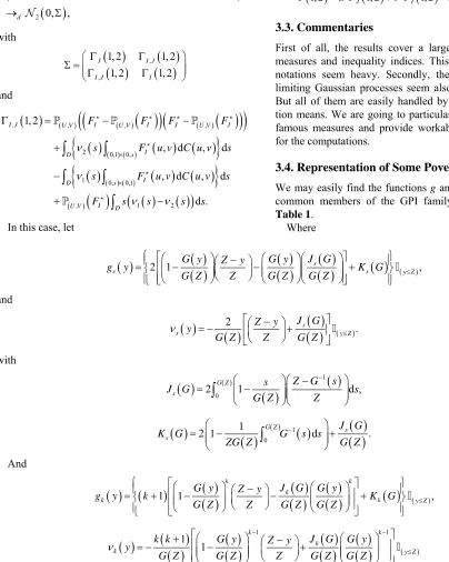
Table 3. Variations of the inequality indices.
Indice I 1,2 I 1,2 CI95%
I 1,2
GE (0.5) −0.04025832 0.01770106 [−0.05588673; −0.03611789]
GE (2) −0.06408679 0.07224733 [−0.09545863; −0.05552007]
GE (3) −0.1008038 0.1205114 [−0.1495352; −0.09795348]
THEIL −0.04569319 0.02223474 [−0.0635651; −0.04140879]
MLD −0.03645671 0.01523784 [−0.05085476; −0.03251291]
ATK (0.5) −0.01976068 0.004225092 [−0.02742201; −0.01776374]
ATK (−0.5) −0.04423886 0.02212773 [−0.06159485; −0.03949192]
Table 4. Variations of the poverty indices.
Ratio J 1,2 J 1,2 CI95%
J 1,2
SHOR −0.03024621 0.02353406 [−0.04264967; −0.01985518]KAK (1) −0.02108905 0.01097123 [−0.02982085; −0.01425729]
KAK (2) −0.02055594 0.01007820 [−0.02961271; −0.01469601]
FGT (0) −0.05977098 0.3170756 [−0.09355847; −0.009889805]
FGT (1) −0.01859332 0.00922992 [−0.02620413; −0.01192899]
[image:8.595.101.497.241.383.2]FGT (2) −0.00432289 0.0008381113 [−0.007194404; −0.002892781]
Table 5. Ratio of the variations with Shorrocks measure.
Ratio R 1,2 IJ 1,2 1,2 CI95%
R 1,2
SHOR/GE (0.5) 0.7513034 0.005477263 15.60737 [0.3858608; 0.9728719]
SHOR/GE (2) 0.471957 0.006487665 8.157275 [0.2018082; 0.6261873]
SHOR/GE (3) 0.3000503 0.009018111 2.851175 [0.1271085; 0.3780043]
SHOR/THEIL 0.6619413 0.005642781 12.36007 [0.3342390; 0.8566255]
SHOR/MLD 0.8296473 0.8296473 18.77303 [0.4278509; 1.071647]
SHOR/ATK (0.5) 1.530626 0.002695030 64.49043 [0.7866646; 1.979908]
SHOR/ATK (−0.5) 0.6837023 0.007288597 12.21780 [0.555278; 1.395697]
SHOR/CHAMP 0.8839194 0.005165236 20.86647 [0.4634852; 1.142229]
Table 6. Ratio of the variations with Sen measure.
Ratio R 1,2 IJ 1,2 1,2 CI95%
R 1,2
SEN/GE (0.5) 0.3290702 0.003112166 7.754599 [0.272201; 0.6859714]SEN/GE (2) 0.3290702 0.003512353 4.013294 [0.1431155; 0.4407834]
SEN/GE (3) 0.2092089 0.005939808 1.354192 [0.0916464; 0.2645570]
SEN/THEIL 0.461536 0.003364929 6.035583 [0.237376; 0.6024165]
SEN/MLD 0.5784683 0.002968939 9.506736 [0.2996504; 0.7577893]
SEN/ATK (0.5) 1.067223 0.001542060 31.99108 [0.555278; 1.395697]
SEN/ATK (−0.5) 0.4360427 0.003368434 6.534366 [0.2461303; 0.625955]
SEN/CHAMP 0.6163094 0.003038844 10.33521 [0.3273292; 0.8050137]
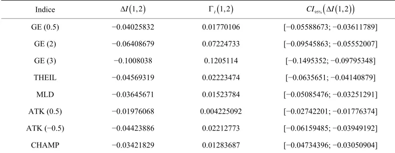
Table 7. Ratio of the variations with Kakwani (2) measure.
Ratio R 1,2 IJ 1,2 1,2 CI95%
R 1,2
KAK (2)/GE (0.5) 0.510601 0.002574653 7.443462 [0.2788993; 0.6842854]KAK (2)/GE (2) 0.3207516 0.008486058 2.93814 [0.1661299; 0.4208233]
KAK (2)/GE (3) 0.2039203 0.005185377 1.276858 [0.09508295; 0.2629838]
KAK (2)/THEIL 0.4498688 0.002906321 5.72986 [0.2442552; 0.5999303]
KAK (2)/MLD 0.5638451 0.002365820 9.220372 [0.3058926; 0.7570787]
KAK (2)/ATK (0.5) 1.040245 0.001292464 30.63183 [0.5694048; 1.391776]
KAK (2)/ATK (−0.5) 0.4646579 0.001933209 6.672792 [0.2464103; 0.630237]
[image:8.595.99.497.411.559.2] [image:8.595.101.496.587.735.2]Table 8. Ratio of the variations with FGT (1) measure.
Ratio R 1,2 IJ 1,2 1,2 CI95%
R 1,2
FGT (1)/GE (0.5) 0.4618504 0.003359959 6.109622 [0.2308332; 0.5981059]
FGT (1)/GE (2) 0.29901272 0.004159761 3.140289 [0.2316082; 0.4949175]
FGT (1)/GE (3) 0.1844506 0.005815332 1.100702 [0.0761356; 0.2320249]
FGT (1)/THEIL 0.4069167 0.003487018 4.824886 [0.2000723; 0.5264534]
FGT (1)/MLD 0.5100109 0.003329621 7.371324 [0.2557003; 0.6591174]
FGT (1)/ATK (0.5) 0.9409253 0.001652060 25.25488 [0.4705622; 1.217276]
FGT (1)/ATK (−0.5) 0.4202938 0.004429351 4.81098 [0.2142764; 0.5401868]
[image:9.595.99.498.277.425.2]FGT (1)/CHAMP 0.5433737 0.003126249 8.218207 [0.2768286; 0.7027897]
Table 9. Ratio of the variations with FGT (0) measure.
Ratio R 1,2 IJ 1,2 1,2 CI95%
R 1,2
FGT (0)/GE (0.5) 1.484686 1.484686 192.9616 [0.09236428; 2.156398]
FGT (0)/GE (2) 0.9326567 0.02159780 82.69382 [0.009587167; 1.360782]
FGT (0)/GE (3) 0.5929437 0.03215672 31.62072 [0.0002219161; 0.8357621]
FGT (0)/THEIL 1.308094 0.01626234 149.7108 [0.07643712; 1.894496]
FGT (0)/MLD 1.639505 0.01332770 236.7108 [0.09833456; 2.383401]
FGT (0)/ATK (0.5) 3.024743 0.00717539 799.837 [0.1882737; 4.390527]
FGT (0)/ATK (−0.5) 1.351097 0.01606948 160.4669 [0.08224307; 1.964480]
[image:9.595.99.497.453.601.2]FGT (0)/CHAMP 1.746755 0.01248913 266.9863 [0.1148277; 2.542700]
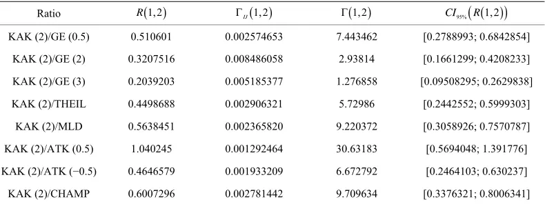
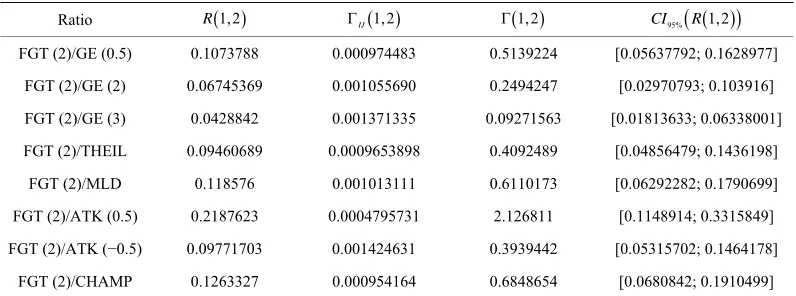
Table 10. Ratio of the variations with FGT (2) measure.
Ratio R 1,2 IJ 1,2 1,2 CI95%
R 1,2
FGT (2)/GE (0.5) 0.1073788 0.000974483 0.5139224 [0.05637792; 0.1628977]
FGT (2)/GE (2) 0.06745369 0.001055690 0.2494247 [0.02970793; 0.103916]
FGT (2)/GE (3) 0.0428842 0.001371335 0.09271563 [0.01813633; 0.06338001]
FGT (2)/THEIL 0.09460689 0.0009653898 0.4092489 [0.04856479; 0.1436198]
FGT (2)/MLD 0.118576 0.001013111 0.6110173 [0.06292282; 0.1790699]
FGT (2)/ATK (0.5) 0.2187623 0.0004795731 2.126811 [0.1148914; 0.3315849]
FGT (2)/ATK (−0.5) 0.09771703 0.001424631 0.3939442 [0.05315702; 0.1464178]
FGT (2)/CHAMP 0.1263327 0.000954164 0.6848654 [0.0680842; 0.1910499]
the same for the Shorrocks measure. Lastly, gamma_ mergslo3.dat concerns the kakwani measures. Unless the user uploads new data1.txt and data2.txt files, the out- comes should be the same as those presented in the Appendix.
3.5.2. Analysis
First of all, we find in Tables 3 and 4 in the appendix 5 that at an asymptotical level, all our inequality measures and poverty indices used here have decreased. When
inspecting the asymptotic variance, we see in Table 4 that for the poverty indice, the FGT and the Kakwani classes respectively for 1, 2 and k = 1, k = 2 have the minimum variance, specially for 2 and k = 2. This advocates for the use of the Kakwani and the FGT measures for poverty reduction evaluation. As for the inequality approach in Table 3, it seems that Atkin- son measure ATK (0.5) has the minimum variance and then is recommended.
Table 11. Dependence of over 50%.
Couples (KAK (2), GE (0.5)) (KAK (2), MLD) (FGT (1), CHAMP)
Dependences (%) 51.06 51.06 54.33
Couples (SEN, MLD) (KAK (2), CHAMP) (SEN, CHAMP)
Dependences (%) 57.84 60.07 61.63
Couples (SHOR, THEIL) (SHOR, ATK (−0.5)) (SHOR, GE (0.5))
Dependences (%) 66.19 68.37 75.13
Couples (SHOR, MLD) (SHOR, CHAMP) (SHOR, ATK)
Dependences (%) 82.29 88.39 153.06
measure, we have a dependence of over 50% for the fol- lowing couples in Table 11, that we can find in Tables 5 to 8.
The maximum ratio 3.024 is attained for FGT (0) and Atkinson (0.5). Based on these data, and on the confi- dence intervals in Table 9, we would report at least of 46.43% for these two measures and conclude that the gain over poverty in Senegal between these two periods is significally pro-poor. We would have worked with all couples with a ratio over 50% to have the same conclu-sion.
The present analysis should be developped in a sepa- rated paper research since this one was devoted to a theo- ritical basis. We plan to apply at a regional basis, that is for the countries of the UEMOA in West Africa.
4. Conclusion
We have been able to compute confidence intervals for the ratio of variations for the poverty and the inequality indices. The results enabled us to cheek whether the growth is pro or against poor in Senegal from 2002 to 2006. It always remains to undertake large scale data driven applications at a regional level, precisely in the UEMOA African area. We used in this paper a Theil-like family of inequality measures that does not include the celebrated and important Gini index. Moreover other the Theil-like families exist. It would be interesting to have the same theory developed here using the Gini index and other families as well. We plan to do it in a very close future.
5. Acknowledgements
We express our thanks to the Ministère de l’Enseigne-ment Supérieur et de la Recherche for financial support under a FIRST grant 2013-2014.
REFERENCES
[1] G. S. Lo, S. T. Sall and C. T. Seck, “Une Théorie As- ymptotique des Indicateurs de Pauvreté,” Comptes Ren-
dus Mathématiques de l’Académie des Sciences. Mathe-
matical Reports of the Academy of Canada, Vol. 31, No.
2, 2009, pp. 45-52.
[2] G. S. Lo, “The Generalized Poverty Index,” Far East
Journal of Theoretical Statistics, Vol. 42, No. 1, 2013, pp.
1-22.
[3] B. Zheng, “Aggregate Poverty Measures,” Journal of
Economic Surveys, Vol. 11, No. 2, 1997, pp. 123-162.
doi:10.1111/1467-6419.00028
[4] K. A. Sen, “Poverty: An Ordinal Approach to Measure- ment,” Econometrica, Vol. 44, No. 2, 1976, pp. 219-231. doi:10.2307/1912718
[5] N. Kakwani, “On a Class of Poverty Measures,” Econo-
metrica, Vol. 48, No. 2, 1980, pp. 437-446.
doi:10.2307/1911106
[6] A. Shorrocks, “Revisiting the Sen Poverty Index,” Econo-
metrica, Vol. 63, No. 5, 1995, pp. 1225-1230.
doi:10.2307/2171728
[7] S. Clark, R. Hemming and D. Ulph, “On Indices for the Measurement of Poverty,” Economic Journal, Vol. 91,
1981, pp. 525-526. doi:10.2307/2232600
[8] J. E. Foster, J. Greer and E. Thorbecke, “A Class of De- composable Poverty Measures,” Econometrica, Vol. 52,
No. 3, 1984, pp. 761-766. doi:10.2307/1913475
[9] S. T. Sall and G. S. Lo, “The Asymptotic Theory of the Poverty Intensity in View of Extreme Values Theory for Two Simple Cases,” Afrika Statistika, Vol. 2, No. 1, 2007,
pp. 41-55.
[10] S. T. Sall and G. S. Lo, “Uniform Weak Convergence of the Time-Dependent Poverty Measure for Continuous Longitudinal Data,” Brazilian Journal of Probability and
Statistics, Vol. 24, No. 3, 2010, pp. 457-467.
doi:10.1214/08-BJPS101
[11] F. A. Cowell, “Theil, Inequality and the Structure of In- come Distribution,” London School of Economics and Political Sciences, London, 2003.
doi:10.1016/0014-2921(80)90051-3
[12] H. Theil, “Economics and Information Theory,” North Holland, Amsterdam, 1967.
[13] F. A. Cowell, “Generalized Entropy and the Measurement of Distributional Change,” European Economic Review,
Vol. 13, No. 1, 1980, pp. 147-159.
nal of Economic Theory, Vol. 2, No. 3, 1970, pp. 244-
263. doi:10.1016/0022-0531(70)90039-6
[15] D. G. Champernowne and F. A. Cowell, “Economic Ine- quality and Income Distribution,” Cambridge University Press, Cambridge, 1998.
[16] S. Kolm, “Unequal Inequalities I,” Journal of Economic
Theory, Vol. 12, No. 3, 1976, pp. 416-442.
doi:10.1016/0022-0531(76)90037-5
[17] A. K. Sen, “On Economic Inequality,” Clarendon Press, Oxford, 1973. doi:10.1093/0198281935.001.0001
[18] J. C. Harsanyi, “Cardinal Utility in Welfare Economics of Concentration,” Journal of the Royal Statistical Society,
Series A, Vol. 123, 1953, pp. 423-434.
[19] J. C. Harsanyi, “Cardinal Welfare, Individualistic Ethics and Interpersonal Comparisons of Utility,” Journal of
Po-litical Economy, Vol. 63, No. 4, 1955, pp. 309-321.
doi:10.1086/257678
[20] M. Rothschild and J. E. Stiglitz, “Some Further Results on the Measurement of Inequality,” Journal of Economic
Theory, Vol. 6, 1973, pp. 188-203.
doi:10.1016/0022-0531(73)90034-3
[21] L. S. Temkin, “Inequality,” Oxford University Press, Ox- ford, 1993.
[22] S. Kullback, “Inference Theory and Statistics,” John Wiley, New York, 1959.
[23] F. A. Cowell, “On the Structure of Additive in Equality Measures,” Review of Economic Studies, Vol. 47, No. 3,
1980, pp. 521-531. doi:10.2307/2297303
[24] F. A. Cowell, “Measurement of Inequality,” In: A. B. Atkinson and F. Bourguignon, Eds., Handbook of Income
Distribution, 2000, pp. 87-166.
doi:10.1016/S1574-0056(00)80005-6
[25] G. S. Lo and S. T. Sall, “Asymptotic Representation Theorems for Poverty Indices,” Afrika Statistika, Vol. 5,
1996, pp. 238-244.
[26] A. W. Van der Vaart and J. A. Wellner, “Weak Conver- gence and Empirical Processes: With Applications to Sta- tistics,” Springer-Verlag, New York, 1996.
doi:10.1007/978-1-4757-2545-2
[27] G. R. Shorack and J. A. Wellner, “Empirical Processes with Applications to Statistics,” Wiley-Interscience, New York, 1986.
[28] G. S. Lo, “A Simple Note on Some Empirical Stochastic Process as a Tool in Uniform L-Statistics Weak Laws,”
Appendix
Proofs of the Theorems Proof of Theorem 2.
By using the delta-method, we have for all i
1, 2 :
1 1 1 1
1
1 , 1
1
1
1 1
1 , 1
n
i i
n n p j
j n
i j j U V i p n i p
j
n h i h i h i n i i o h i X X o
n
h i f U V f o h i f o
n
1 .
j p
Then
1 n 1
n
1
i
1 .n h i h i h i f op (6)
Similarly, we have
2 n 2
n
2
i
1 .n h i h i h i f op (7)
From this and (3.1), we have
,
,
,
1 1
1 n 1 n , ;
i i
n j j i h j j U V
j j
n B i B i h X h X f U V f
n n
i hand then
n
n
, .n B i B i fi h (8)
Further
2 2
1 1
2 2
1 1
1 .
n
n n
n
n
i n
n
B i B i
n I i I i n h i h i
h i h i
B i B i
K n h i h i o
h i h i
p
But
2 2
1 1
1
2
1 1 1
1
, 2
1 1 1
1
, 2 2
1 1
1
1 1
1
1 .
n
n n
n
n p
n n
n i h n i p
n n
n i h i p
B i B i
n h i h i
h i h i
n B i B i B i h i
h i n i i o
h i h i h i
B i h i
f h i f o
h i h i h i
B i h i
f h i f o
h i h i
Thus
1
, 2 2
1 1
1
1 ,
n i n i h i
B i h i
n I i I i K f h i f o
h i h i
p
that is