Munich Personal RePEc Archive
Two Sample Tests for High Dimensional
Covariance Matrices
Li, Jun and Chen, Songxi
4 May 2012
Two Sample Tests for High Dimensional Covariance
Matrices
Jun Li and Song Xi Chen
Department of Statistics, Iowa State University; and
Department of Business Statistics and Econometrics
and Center for Statistical Science, Peking University
and Department of Statistics, Iowa State University
email: [email protected], [email protected]
May 4, 2012
Abstract
We propose two tests for the equality of covariance matrices between two high-dimensional
populations. One test is on the whole variance-covariance matrices, and the other is on
off-diagonal sub-matrices which define the covariance between two non-overlapping segments of
the high-dimensional random vectors. The tests are applicable (i) when the data dimension
is much larger than the sample sizes, namely the “large p, small n” situations and (ii) without
assuming parametric distributions for the two populations. These two aspects surpass the
capability of the conventional likelihood ratio test. The proposed tests can be used to test
on covariances associated with gene ontology terms.
Keywords: High dimensional covariance; Large p small n; Likelihood ratio test; Testing
1. INTRODUCTION
Modern statistical data are increasingly high dimensional, but with relatively small sample
sizes. Genetic data typically carry thousands of dimensions for measurements on the genome.
However, due to limited resources available to replicate study objects, the sample sizes are
usually much smaller than the dimension. This is the so-called “large p, small n” paradigm.
An enduring interest in Statistics is to know if two populations share the same distribution
or certain key distributional characteristics, for instance the mean or covariance. The two
populations here can refer to two “treatments” in a study. As testing for equality of
high-dimensional distributions is far more challenging than that for the fixed-high-dimensional data,
testing for equality of key characteristics of the distributions is more achievable and desirable
due to easy interpretation. There has been a set of research on inference for means of
high-dimensional distributions either in the context of multiple testing as in van der Laan and
Bryan (2001), Donoho and Jin (2004), Fan, Hall, and Yao (2007), and Hall and Jin (2008),
or in the context of simultaneous multivariate testing as in Bai and Saranadasa (1996) and
Chen and Qin (2010). See also Huang, Wang, and Zhang (2005), Fan, Peng, and Huang
(2005) and Zhang and Huang (2008) for inference on high-dimensional conditional means.
In addition to detecting difference among the population means, there is a strong
mo-tivation for comparing dependence among components of random vectors under different
treatments, as high data dimensions can potentially increase the complexity of the
depen-dence. In genomic studies, genetic measurements, either the micro-array expressions or the
single nucleotide polymorphism (SNP) counts, may have an internal structure dictated by
the genetic networks of living cells. And the variations and dependence among the
measure-ments of the genes may be different under different biological conditions and treatmeasure-ments.
For instance, some genes may be tightly correlated in the normal or less severe conditions,
but they can become decoupled due to certain disease progression; see Shedden and Taylor
(2004) for a discussion.
probability limits and the limiting distributions of extreme eigenvalues of the sample
covari-ance matrix based on the random matrix theory are developed in Bai (1993), Bai and Yin
(1993), Tracy and Widom (1996), Johnstone (2001) and El Karoui (2007), Johnstone and
Lu (2009), Bai and Silverstein (2010) and others. Wu and Pourahmadi (2003) and Bickel
and Levina (2008a, 2008b) proposed consistent estimators to the population covariance
ma-trices by either truncation or Cholesky decomposition. Fan, Fan and Lv (2008), Lam and
Yao (2011) and Lam, Yao and Bathia (2011) considered covariance estimation under factor
models. There are also developments in conducting LASSO-type regularization estimation
of high-dimensional covariances in Huang, Liu, Pourahmadi and Liu (2006) and Rothman,
Levina and Zhu (2010). Despite these developments, it is still challenging to transform these
results to test procedures on high-dimensional covariance matrices.
As part of the effort in discovering significant differences between two high-dimensional
distributions, we develop in this paper two-sample test procedures on high-dimensional
co-variance matrices. Let Xi1, ..., Xini be an independent and identically distributed sample
drawn from a p-dimensional distribution Fi, for i = 1 and 2 respectively. Here the
dimen-sionality p can be a lot larger than the two sample sizes n1 and n2 so that p/ni → ∞.
Let µi and Σi be, respectively, the mean vector and variance-covariance matrix of the ith
population. The primary interest is to test
H0a: Σ1 = Σ2 versus H1a: Σ1 ̸= Σ2. (1.1)
Testing for the above high-dimensional hypotheses is a non-trivial statistical problem.
De-signed for fixed-dimensional data, the conventional likelihood ratio test (see Anderson (2003)
for details) may be used for the above hypothesis underp≤min{n1, n2}. If we let
¯ Xi =
1 ni
ni ∑
j=1
Xij and Qi = ni ∑
j=1
(Xij −X¯i)(Xij −X¯i)′,
then the likelihood ratio (LR) statistic for H0a is
λn=
∏2
i=1|Qi|
1 2ni
|Q|12n
n12pn
∏2
i=1n
1 2pni
where Q = Q1 +Q2 and n = n1 +n2. However, when p > min{n1, n2}, at least one of
the sample covariance matrices Qi/(ni−1) is singular (Dykstra 1970). This causes the LR
statistic−2 log(λn) to be either infinite or undefined, which fundamentally alters the limiting
behavior of the LR statistic. In an important development, Bai et al. (2009) demonstrated
that, even when p≤min{n1, n2} where λn is properly defined, the test encounters a power
loss if p → ∞ in such a manner that p/ni → ci ∈ (0,1) for i = 1 and 2. By employing
the theory of large dimensional random matrices, Bai et al. (2009) proposed a correction to
the LR statistic and demonstrated that the corrected test is valid under p/ni →ci ∈(0,1).
Schott (2007) proposed a test based on a metric that measures the difference between the two
sample covariance matrices by assuming p/ni → ci ∈ [0,∞) and the normal distributions.
There are also one sample tests for a high-dimensional variance-covariance Σ. Ledoit and
Wolf (2002) introduced tests for Σ being sphericity and identity for normally distributed
random vectors. Ledoit and Wolf (2004) considered a class of covariance estimators which
are convex sums of Sn and Ip under moderate dimensionality (p/n → c). Cai and Jiang
(2011) developed tests for Σ having a banded diagonal structure based on random matrix
theory. Lan et al. (2010) developed a bias-corrected test to examine the significance of
the off-diagonal elements of the residual covariance matrix. All these tests assume either
normality or moderate dimensionality such that p/n→cfor a finite constant c, or both.
We develop in this paper two-sample tests on high-dimensional variance-covariances
with-out the normality assumption while allowing the dimension to be much larger than the sample
sizes. In addition to testing for the whole variance-covariance matrices, we propose a test
on the equality of off-diagonal sub-matrices in Σ1 and Σ2. The interest on such a test arises
naturally in applications, when we are interested in knowing if two segments of the
high-dimensional data share the same covariance between the two treatments. We will argue in
Section 3 that the two tests on the whole covariance and the off-diagonal sub-matrices may
be used collectively to reduce the dimensionality of the testing problem.
This paper is organized as follows. We propose the two-sample test for the whole
and a power evaluation. Properties of the test for the off-diagonal sub-matrices are reported
in Section 3. Results from simulation studies are outlined in Section 4. Section 5
demon-strates how to apply the proposed tests on a gene ontology data set for acute lymphoblastic
leukemia. All technical details are relegated to Section 6.
2. TEST FOR HIGH DIMENSIONAL VARIANCE-COVARIANCE
The test statistic for the hypothesis (1.1) is formulated by targeting on tr{(Σ1−Σ2)2}, the
squared Frobenius norm of Σ1 −Σ2. Although the Frobenius norm is large in magnitude
compared with other matrix norms, using it for testing brings two advantages. One is that
test statistics based on the norm are relatively easier to be analyzed than those based on
the other norm, which is especially the case when considering the limiting distribution of
the test statistics. The latter renders formulations of test procedures and power analysis, as
we will demonstrate later. The other advantage is that it can be used to directly target on
certain sections of the covariance matrix as shown in the next section. The latter would be
hard to accomplish with other norms.
As tr{(Σ1−Σ2)2}=tr(Σ21) +tr(Σ22)−2tr(Σ1Σ2), we will construct estimators for each
term. It is noted that tr(S2
nh), where Snh is the sample covariance of the hth sample, is a poor estimator of tr(Σ2
h) under high dimensionality. The idea is to streamline terms in
tr(S2
nh) so as to make it unbiased to tr(Σ2h) and easier to analyze in subsequent asymptotic evaluations. We consider U-statistics of form 1
nh(nh−1) ∑
i̸=j(Xhi′ Xhj)2 which is unbiased if µh = 0. To account for µh ̸= 0, we subtract two other U-statistics of order three and four
respectively, using an approach dated back to Glasser (1961, 1962). Specifically, we propose
Anh =
1 nh(nh−1)
∑
i̸=j
(Xhi′ Xhj)2− 2
nh(nh−1)(nh−2) ⋆
∑
i,j,k
Xhi′ XhjXhj′ Xhk
+ 1
nh(nh−1)(nh−2)(nh−3) ⋆
∑
i,j,k,l
Xhi′ XhjXhk′ Xhl (2.1)
to estimate tr(Σ2
h). Throughout this paper we use
∑⋆
to denote summation over mutually
Similarly, the estimator for tr(Σ1Σ2) is
Cn1n2 =
1 n1n2
∑
i
∑
j (X′
1iX2j)2−
1 n1n2(n1−1)
⋆
∑
i,k
∑
j X′
1iX2jX2′jX1k
− 1
n1n2(n2−1)
⋆
∑
i,k
∑
j X′
2iX1jX1′jX2k
+ 1
n1n2(n1−1)(n2−1)
⋆
∑
i,k ⋆
∑
j,l X′
1iX2jX1′kX2l. (2.2)
There are other ways to attain estimators for tr(Σ2
h) and tr(Σ1Σ2). In fact, there is a
family of estimators for tr(Σ2
h) in the form of tr(Sh2)−αnh ∑nh
i=1tr{(XhiXhi′ −Sh)2} where αnh =α/n
2
h for any constant α. A family can be similarly formulated for tr(Σ1Σ2). It can
be shown that this family of estimators is asymptotically equivalent to the proposed Anh in
the sense that they share the same leading order term. However, this family is more complex
than the proposed.
The test statistic is
Tn1,n2 =An1 +An2 −2Cn1n2 (2.3)
which is unbiased for tr{(Σ1 −Σ2)2}. Besides the unbiasedness, Tn1,n2 is invariant under
the location shift and orthogonal rotation. This means that we can assume without loss of
generality that E(Xij) = 0 in the rest of the paper. As noted by a reviewer, the computation
ofTn1,n2 would be extremely heavy if the sample sizesnh are very large. Indeed, the
compu-tation burden comes from the last two sums in Anh and the last three in Cn1,n2, where the
numbers of terms in the summations are in the order of n3
h orn4h, respectively. Although the main motivation was the “large p small n” situations, we nevertheless require nh → ∞ in
our asymptotic justifications. A solution to alleviate the computation burden can be found
by noting that, the last two terms inAnh and the last three inCn1,n2 are all of smaller order
than the first, under the assumption of µh = 0. This means that we can first transform each
datum Xhi to Xhi−Xn¯ h, and then compute only the first term in (2.1) and (2.2). These
will reduce the computation toO(n2
h) without affecting the asymptotic normality. The only
To establish the limiting distribution of Tn1,n2 so as to establish the two sample test for
the variance-covariance, we assume the following conditions.
A1. As min{n1, n2} → ∞, n1/(n1+n2)→ρ for a fixed constantρ∈(0,1).
A2. As min{n1, n2} → ∞,p=p(n1, n2)→ ∞, and for anyk andl ∈ {1,2},tr(ΣkΣl)→
∞ and
tr{(ΣiΣj)(ΣkΣl)}=o{tr(ΣiΣj)tr(ΣkΣl)}. (2.4)
A3. For each i = 1 or 2, Xij = ΓiZij +µi where Γi is a p× mi matrix such that ΓiΓ′i = Σi, {Zij}nj=1i are independent and identically distributed (i.i.d.) mi-dimensional
random vectors with mi ≥ p and satisfy E(Zij) = 0, Var(Zij) = Imi, the mi×mi identity
matrix. Furthermore, if write Zij = (zij1, ..., zijmi)
′, then each zijk has finite 8th moment,
E(z4
ijk) = 3 + ∆i for some constant ∆i and for any positive integers q and αl such that
∑q
l=1αl ≤8 E(z
α1
ijl1...z
αq
ijlq) = E(z
α1
ijl1)...E(z
αq
ijlq) for any l1 ̸=l2 ̸=...̸=lq.
While Condition A1 is of standard for two-sample asymptotic analysis, A2 spells the
extent of high dimensionality and the dependence which can be accommodated by the
pro-posed tests. A key aspect is that it does not impose any explicit relationships between p
and the sample sizes, but rather requires a quite mild (2.4) regarding the covariances. To appreciate (2.4), we note that ifi=j =k =l, it has the form oftr(Σ4
i) = o{tr2(Σ2i)}, which is valid if all the eigenvalues of Σi are uniformly bounded. Condition (2.4) also makes the asymptotic study of the test statistic manageable under high dimensionality. We note here
that requiring tr(ΣkΣl) → ∞ is a precursor to (2.4). We do not assume specific paramet-ric distributions for the two samples. Instead, a general multivariate model is assumed in
A3 which was advocated in Bai and Saranadasa (1996) for testing high dimensional means.
The model resembles that of the factor model with Zi representing the factors, except that
here we allow the number of factor mi at least as large as p. This provides flexibility in
accommodating a wider range of multivariate distributions for the observed data Xij.
variance of Tn1,n2 under either H0a orH1a is
σ2n1,n2 =
2 ∑
i=1 [
4 n2
i
tr2(Σ2i) + 8 nitr{(Σ
2
i −Σ1Σ2)2}
+ 4∆i ni tr{Γ
′
i(Σ1−Σ2)Γi◦Γ′i(Σ1−Σ2)Γi}
]
+ 8 n1n2
tr2(Σ1Σ2) (2.5)
whereA◦B = (aijbij) for two matricesA= (aij) andB = (bij). Note that for any symmetric
matrix A, tr(A◦A)≤tr(A2). Hence,
tr{Γ′1(Σ1−Σ2)Γ1◦Γ′1(Σ1−Σ2)Γ1} ≤tr{(Σ21−Σ1Σ2)2} and
tr{Γ′
2(Σ1−Σ2)Γ2◦Γ′2(Σ1−Σ2)Γ2} ≤tr{(Σ22−Σ2Σ1)2}.
These together with the fact that ∆i ≥ −2 ensure that σ2
n1,n2 > 0. We note that the
Γi-Zij pair in Model A3 is not unique, and there are other pairs, say ˜Γi and ˜Zij, such that
Xij = ˜ΓiZij˜ . However, it can be shown that the value of 4∆in
i tr{Γ
′
i(Σ1−Σ2)Γi◦Γ′i(Σ1−Σ2)Γi}
remains the same.
The following theorem establishes the asymptotic normality of Tn1,n2.
Theorem 1. Under Conditions A1-A3, as min{n1, n2} → ∞
σn−11,n2
[
Tn1,n2 −tr{(Σ1 −Σ2)
2
}
]
d
−
→N(0,1).
It is noted that under H0a : Σ1 = Σ2 = Σ, say, σ2n1,n2 becomes
σ02,n1,n2 = 4( 1 n1
+ 1 n2
)2tr2(Σ2).
To formulate a test procedure, we need to estimate σ2
0,n1,n2. As An1 and An2 are unbiased
estimators of tr(Σ2
1) and tr(Σ22), respectively, we will use ˆσ02,n1,n2 =:
2
n2An1 +
2
n1An2 as the
estimator. The following theorem shows that ˆσ2
0,n1,n2 is ratio-consistent to σ
2 0,n1,n2.
Theorem 2. Under Conditions A1-A3 and H0a, as min{n1, n2} → ∞,
Ani
tr(Σ2
i) p
−
→1 for i= 1 and 2, and σˆ0,n1,n2
σ0,n1,n2
p
−
→1. (2.6)
Applying Theorems 1 and 2, under H0a : Σ1 = Σ2,
Ln= Tn1,n2
ˆ σ0,n1,n2
d
−
Hence, the proposed test with a nominal α level of significance rejects H0a if Tn1,n2 ≥
ˆ
σ0,n1,n2zα, where zα is the upper-α quantile of N(0,1).
Let β1,n1,n2(Σ1,Σ2;α) = P(Tn1,n2/ˆσ0,n1,n2 > zα|H1a) be the power of the test under H1a:
Σ1 ̸= Σ2. From Theorems 1 and 2, the leading order power is
Φ
(
−Zn
1,n2(Σ1,Σ2)zα+
tr{(Σ1−Σ2)2}
σn1,n2
)
, (2.8)
where Zn
1,n2(Σ1,Σ2) = (σn1,n2)
−1{ 2
n2tr(Σ
2
1) + n21tr(Σ
2
2)}. It is the case that Zn1,n2(Σ1,Σ2)
is bounded. To appreciate this, we note that σ2
n1,n2 ≥
4
n2 1tr
2(Σ2 1) + n42
2tr
2(Σ2
2). Let γp =
tr(Σ2
1)/tr(Σ22) and kn =n1/(n1+n2), then
Zn
1,n2(Σ1,Σ2) ≤
2
n2tr(Σ
2
1) + n21tr(Σ
2 2) √ 4 n2 1tr
2(Σ2 1) + n42
2tr
2(Σ2 2)
=:Rn(γp),
where Rn(u) = ( kn
1−knu+ 1){u
2+ ( kn
1−kn)
2}−1/2. Since Rn(u) is maximized uniquely at u∗ =
( kn 1−kn)
3, Z
n1,n2(Σ1,Σ2)≤
1
kn(1−kn). Thus,
β1,n1,n2(Σ1,Σ2;α)≥Φ
(
−k zα
n(1−kn)
+ tr{(Σ1−Σ2)
2}
σn1,n2
)
(2.9)
implying the power is bounded from below by the probability on the right-hand side.
Both (2.8) and (2.9) indicate that SNR1(Σ1,Σ2) =:tr{(Σ1−Σ2)2}/σn1,n2 is instrumental
in determining the power of the test. We term SNR1(Σ1,Σ2) as the signal-to-noise ratio for
the current testing problem since tr{(Σ1−Σ2)2} may be viewed as the signal while σn1,n2
may be viewed as the level of the noise. If the signal is strong or the noise is weak so that
the to-noise ratio diverges to the infinity, the power will converge to 1. If the
signal-to-noise ratio diminishes to 0, the test will not be powerful and cannot distinguish H0afrom
H1a. We note that
σ2n1,n2 ≤ 4{ 1
n1
tr(Σ21) + 1 n2
tr(Σ22)}2
+ max{8 + 4∆1,8 + 4∆2}{
1 n1
tr(Σ21) + 1 n2
tr(Σ22)}tr{(Σ1−Σ2)2}.
Let δ1,n ={n11tr(Σ21) + n12tr(Σ
2
2)}/tr{(Σ1 −Σ2)2}, then
SNR1(Σ1,Σ2)≥ [
4δ12,n+ max{8 + 4∆1,8 + 4∆2}δ1,n
Thus, if the difference between Σ1 and Σ2 is not too small so that
tr{(Σ1−Σ2)2} is at the same or a larger order of (2.10)
1 n1
tr(Σ21) + 1 n2
tr(Σ22),
the test will be powerful. Condition (2.10) is trivially true for fixed-dimensional data while ni → ∞. For high-dimensional data, it is less automatic as tr(Σ2i) can diverge. To gain
further insight on (2.10), letλi1 ≤λi2 ≤ · · · ≤λipbe the eigenvalues of Σi. Then, a sufficient
condition for the test to have a non-trivial power is tr{(Σ1 − Σ2)2} = O{n11 ∑pi=1λ21i +
1
n2
∑p
i=1λ22i}. If all the eigenvalues of Σ1 and Σ2 are bounded away from zero and infinity,
(2.10) becomes tr{(Σ1 −Σ2)2} = O(n−1p). Let δβ = p−1 √
tr{(Σ1−Σ2)2} be the average
signal. Then the test has non-trivial power if δβ is at least at the order of n−1
2p−12, which
is actually smaller than the conventional order of n−1/2 for fixed-dimension situations. This
partially reflects the fact that high data dimensionality is not entirely a curse as there are
more data information available as well. If the covariance matrix is believed to have certain
structure, for instance banded or bandable in the sense of Bickel and Levina (2008a), we
may modify the test statistic so that the comparison of the two covariance matrices is made
in the “important regions” under the structure. The modification can be in the form of
thresholding, a topic we would not elaborate in this paper; see Cai, Liu and Xia (2011) for
research in this direction.
3. TEST FOR COVARIANCE BETWEEN TWO SUB-VECTORS
LetXij = (Xij(1), X
(2)
ij ) be a partition of the original data vector into sub-vectors of dimensions
of p1 and p2, and Σi,12 = Cov(Xij(1), X
(2)
ij ) be the covariance between the sub-vectors. The
focus in this section is to develop a test procedure for H0b : Σ1,12 = Σ2,12. Testing for such
a hypothesis is importance in its own right, for instance in detecting changes in correlation
between two groups of genes under two treatment regimes. It can be also viewed as part
To elaborate on this, consider the partition of Σi,
Σi =
Σi,11 Σi,12
Σ′
i,12 Σi,22
(3.1)
induced by the partition of the data vectors. Instead of testing on the whole matrices
Σ1 = Σ2, we can first test separately on the two diagonal blocks Σ1,ll = Σ2,ll forl = 1 and 2,
by employing the test developed in the previous section based on the sub-vectors of the two
sample data respectively. Then, we can test for the off-diagonal blocks H0b : Σ1,12 = Σ2,12
using a test procedure to be developed in this section.
The partition of data vectors also induces a partition of the multivariate model in A3 so
that
Xij(1) = Γ(1)i Zij +µ(1)i and Xij(2) = Γ(2)i Zij +µ(2)i , (3.2)
where Γ(1)i isp1×mi and Γi(2) is p2×mi such that Γ′i = (Γ
(1)
i
′
,Γ(2)i ′) and Γ(1)i Γ(2)i ′ = Σi,12.
We are interested in testing H0b : Σ1,12 = Σ2,12 vs H1b : Σ1,12 ̸= Σ2,12. The test statistic
is aimed at
tr{(Σ1,12−Σ2,12)(Σ1,12−Σ2,12)′}
= tr(Σ1,12Σ′1,12) +tr(Σ2,12Σ′2,12)−2tr(Σ1,12Σ′2,12), (3.3)
a discrepancy measure between Σ1,12 and Σ2,12.
With the same considerations as those when we proposed the estimators in (2.1) and
(2.2), we estimate tr(Σh,12Σ′h,12) by
Unh =
1 nh(nh−1)
∑
i̸=j
Xhi(1)′Xhj(1)Xhj(2)′Xhi(2)
− 2
nh(nh−1)(nh−2) ⋆
∑
i,j,k
Xhi(1)′Xhj(1)Xhj(2)′Xhk(2)
+ 1
nh(nh−1)(nh−2)(nh−3) ⋆
∑
i,j,k,l
and estimatetr(Σ1,12Σ′2,12) by
Wn1n2 =
1 n1n2
∑
i,j
X1(1)i ′X2(1)j X2(2)j ′X1(2)i
− 1
n1n2(n1−1) ∑
i̸=k,j
X1(1)i ′X2(1)j X2(2)j ′X1(2)k
− 1
n1n2(n2−1) ∑
i̸=k,j
X2(1)i ′X1(1)j X1(2)j ′X2(2)k
+ 1
n1n2(n1−1)(n2−1) ∑
i̸=k,j̸=l
X1(1)i ′X2(1)j X1(2)k′X2(2)l . (3.5)
Both Unh and Wn1n2 are linear combinations of U-statistics.
Combining these estimators together leads to an unbiased estimator oftr{(Σ1,12−Σ2,12)(Σ1,12−
Σ2,12)′},
Sn1,n2 =Un1 +Un2 −2Wn1n2, (3.6)
which is also invariant under the location shift and orthogonal rotations.
To establish the asymptotic normality of Sn1,n2, we need an extra assumption regarding
the off-diagonal sub-matrices.
A4. As min{n1, n2} → ∞, for any i, j, k and l ∈ {1,2}.
tr(Σi,11Σj,12Σk,22Σ′l,12) =o{tr(Σi,11Σj,11)tr(Σk,22Σl,22)}. (3.7)
Derivations leading to (A.5) in Section 6 show that, under A2, A3 and A4, the leading order variance of Sn1,n2 is
ωn21,n2 =
2 ∑
i=1 [
2 n2
i
tr2(Σi,12Σ′i,12) +
2 n2
i
tr(Σ2i,11)tr(Σ2i,22)
+ 4
nitr{(Σi,12Σ
′
1,12−Σi,12Σ′2,12)2}
+ 4
nitr{(Σi,11Σ1,12−Σi,11Σ2,12)(Σi,22Σ
′
1,12−Σi,22Σ′2,12)}
+ 4∆i ni tr{Γ
(1)
i
′
(Σ1,12−Σ2,12)Γ(2)i ◦Γ
(1)
i
′
(Σ1,12−Σ2,12)Γ(2)i }
]
+ 4
n1n2
tr2(Σ1,12Σ′2,12) +
4 n1n2
Similarly to the analysis on Tn1,n2 in the previous section, the asymptotic normality of
Sn1,n2 can be established in the following theorem.
Theorem 3. Under Conditions A1-A4, as min{n1, n2} → ∞,
ωn1,n2
−1 [
Sn1,n2 −tr{(Σ1,12−Σ2,12)(Σ1,12−Σ2,12)
′
]
d
−
→N(0,1).
Under H0b: Σ1,12= Σ2,12 = Σ12, say,ωn21,n2 becomes
ω02,n1,n2 = 2( 1 n1
+ 1 n2
)2tr2(Σ12Σ′12) + 2 2 ∑ i=1 1 n2 i
tr(Σ2i,11)tr(Σ2i,22)
+ 4
n1n2
tr(Σ1,11Σ2,11)tr(Σ1,22Σ2,22). (3.9)
In order to formulate a test procedure, ω2
0,n1,n2 needs to be estimated. An unbiased
estimator of tr(Σ2
h,ll) forh= 1 or 2 and l = 1 or 2, is
A(nlh) = 1 nh(nh−1)
∑
i̸=j
(Xhi(l)′Xhj(l))2− 2
nh(nh−1)(nh−2) ⋆
∑
i,j,k
Xhi(l)′Xhj(l)Xhj(l)′Xhk(l)
+ 1
nh(nh−1)(nh−2)(nh−3) ⋆
∑
i,j,k,l
Xhi(l)′Xhj(l)Xhk(l)′Xhl(l).
Similarly, an unbiased estimator of tr(Σ1,hhΣ2,hh), for h= 1 or 2, is
Cn(h1)n2 = 1 n1n2
∑
i,j
(X1(hi)′X2(hj))2− 1 n1n2(n1−1)
∑
i̸=k,j
X1(hi)′X2(hj)X2(hj)′X1(hk)
− n 1
1n2(n2−1) ∑
i̸=k,j
X2(hi)′X1(hj)X1(hj)′X2(hk)
+ 1
n1n2(n1−1)(n2−1) ∑
i̸=k,j̸=l
X1(hi)′X2(hj)X1(hk)′X2(hl).
Then under H0b, an unbiased estimator of ω20,n1,n2 is
c
ω2
0,n1,n2 = 2(
Un1
n2
+ Un2
n1
)2+ 2 n2
1
A(1)n1A(2)n1 + 2 n2
2
A(1)n2A(2)n2 + 4 n1n2
Cn(1)1n2Cn(2)1n2.
The following theorem shows that ωc2
0,n1,n2 is ratio-consistent to ω
2 0,n1,n2.
Theorem 4. Under Conditions A1-A4, and H0b : Σ1,12 = Σ2,12, c
ω2 0,n1,n2
ω2 0,n1,n2
p
Applying Theorems 3 and 4, we have, under H0b,
Sn1,n2
ˆ ω0,n1,n2
d
−
→N(0,1).
This suggests anα-level test that rejectsH0bifSn1,n2 ≥ωˆ0,n1,n2zα. The power of the proposed
test under H1b : Σ1,12 ̸= Σ2,12 is
β2,n1,n2(Σ1,12,Σ2,12;α) =P(Sn1,n2/ˆω0,n1,n2 > zα|H1b).
From Theorems 3 and 4, the leading order power is
Φ
(
− ω˜
ωn1,n2
zα+
tr{(Σ1,12−Σ2,12)(Σ1,12−Σ2,12)′}
ωn1,n2
)
,
where
˜
ω2 = 2{tr(Σ1,12Σ
′
1,12)
n2
+ tr(Σ2,12Σ
′
2,12)
n1 }
2+ 2
n2 1
tr(Σ21,11)tr(Σ21,22)
+ 2 n2
2
tr(Σ2
2,11)tr(Σ22,22) +
4 n1n2
tr(Σ1,11Σ2,11)tr(Σ1,22Σ2,22).
Letηp =tr(Σ1,12Σ′1,12)/tr(Σ2,12Σ′2,12). It may be shown that
˜ ω ωn1,n2
≤
√
R2(ηp) + 1,
where R(γp) is the same function defined in Section 2. Hence, asymptotically,
β2,n1,n2(Σ1,12,Σ2,12;α)
≥ Φ
(
−zα
√
1 +k2
n(1−kn)2 kn(1−kn)
+tr{(Σ1,12−Σ2,12)(Σ1,12−Σ2,12)
′
}
ωn1,n2
)
.
This implies that
SNR2 =:tr{(Σ1,12−Σ2,12)(Σ1,12−Σ2,12)′}/ωn1,n2
is the key quantity that determines the power of the test. Furthermore, let
δ2,n =
1
n1tr(Σ1,11)tr(Σ1,22) +
1
n2tr(Σ2,11)tr(Σ2,22)
tr{(Σ1,12−Σ2,12)(Σ1,12−Σ2,12)′}
It can be shown that
SNR2 ≥ [
4δ22,n+ max{8 + 4∆1,8 + 4∆2}δ2,n
]−12
. (3.10)
Hence, the test is powerful if the difference between Σ1,12 and Σ2,12 is not too small so that
tr{(Σ1,12 −Σ2,12)(Σ1,12 − Σ2,12)′} is at the order of ∑2i=1 n1itr(Σi,11)tr(Σi,22) or larger. A
further analysis on the power, similar to that given at the end of last section, can be made.
Here for the sake of brevity, we will not report.
4. SIMULATION STUDIES
We report results from simulation experiments which were designed to evaluate the
perfor-mance of the two proposed tests. A range of dimensionality and sample sizes was considered
which allowedpto increase as the sample sizes were increased. This was designed to confirm
the asymptotic results reported in the previous sections.
We first considered the test for H0a : Σ1 = Σ2 regarding the whole variance-covariance
matrices. To compare with the conventional likelihood ratio (LR) test and the corrected
LR test proposed by Bai et al. (2009), we first considered cases of p ≤ min{n1, n2} and
the normally distributed data. Specifically, to create the null hypothesis, we simulated both
samples from the p-dimensional standard normal distribution. To evaluate the power of the
three tests, we set the first population to be thep-dimensional standard normally distributed
while simulating the second population according to
Xijk =Zijk+θ1Zijk+1, (4.1)
where{Zijk}were i.i.d. standard normally distributed, andθ1 = 0.5,0.3 and 0.2, respectively.
As θ1 was decreased, the signal strength for the test became weaker. We chose (p, n1, n2) =
(40,60,60),(80,120,120) and (120,180,180), respectively. The empirical size and power for
the three tests are reported in Table 1. All the simulation results reported in this section
were based on 1000 simulations with the nominal significance level to be 5 %.
We then carried out simulations for situations wherep was much larger than the sample
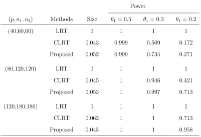
Table 1: Empirical sizes and powers of the conventional likelihood ratio (LR), the corrected
likelihood ratio (CLR) and the proposed tests (Proposed) for the variance-covariance, based
on 1000 replications with normally distributed {Zijk}.
Power
(p, n1, n2) Methods Size θ1 = 0.5 θ1 = 0.3 θ1 = 0.2
(40,60,60) LRT 1 1 1 1
CLRT 0.043 0.999 0.509 0.172
Proposed 0.052 0.999 0.734 0.271
(80,120,120) LRT 1 1 1 1
CLRT 0.045 1 0.946 0.421
Proposed 0.053 1 0.997 0.713
(120,180,180) LRT 1 1 1 1
CLRT 0.062 1 1 0.713
LR tests were no longer applicable. We chose a set of data dimensions from 32 to 700, while
the sample sizes ranged from 20 to 100 respectively. We considered the moving average model
(4.1) with θ1 = 2 as the null model of both populations for size evaluation. To assess the
power performance, the first population was generated according to (4.1) while the second was from
Xijk =Zijk+θ1Zijk+1+θ2Zijk+2, (4.2)
where θ1 = 2 and θ2 = 1. Three combinations of distributions were experimented for the
i.i.d. sequences {Zijk}pk=1 in models (4.1) and (4.2), respectively. They were: (i) both
sequences were the standard normal; (ii) the centralized Gamma(4,0.5) for Sample 1 and
the centralized Gamma(0.5,√2) for Sample 2; (iii) the standard normal for Sample 1 and
the centralized Gamma(0.5,√2) for Sample 2. The last two combinations were designed to
assess the performance under non-normality. The empirical size and power of the test are
reported in Tables 2-4.
We observed from Table 1 that the size of the conventional LR test was grossly distorted,
confirming its breakdown under even mild dimensionality, discovered in Bai et al. (2009).
The severely distorted size for the LR test made its power artificially high. Both the corrected
LR test and the proposed test had quite accurate size approximation to the nominal 5%
level for all cases in Table 1. Both tests enjoyed perfect power at θ1 = 0.5, when the signal
strength of the tests was strong. When the value of θ2 decreased, both tests had smaller
power, although the proposed test was slightly more powerful than the corrected LR test at
θ1 = 0.3 and much more so atθ1 = 0.2, when the signal strength was weaker.
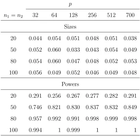
The simulation results for the proposed test with dimensions much larger than the sample
sizes and for non-normally distributed data are reported in Tables 2-4. We note that the LR
tests are not applicable for the setting. The simulation results show that the proposed test
had quite accurate and robust size approximation in a quite wider range of dimensionality
and distributions, considered in the simulation experiments. The tables also show that the
Table 2: Empirical sizes and powers of the proposed test for the variance-covariance matrices,
based on 1000 replications with normally distributed{Zijk} in Models (4.1) and (4.2).
p
n1 =n2 32 64 128 256 512 700
Sizes
20 0.044 0.054 0.051 0.048 0.051 0.038
50 0.052 0.060 0.033 0.043 0.054 0.049
80 0.054 0.060 0.047 0.048 0.052 0.053
100 0.056 0.049 0.052 0.046 0.049 0.048
Powers
20 0.291 0.256 0.267 0.277 0.282 0.291
50 0.746 0.821 0.830 0.837 0.832 0.849
80 0.957 0.992 0.991 0.998 0.999 0.998
100 0.994 1 0.999 1 1 1
the sample sizes became larger.
We then conducted simulations to evaluate the performance of the second test for H0b :
Σ1,12 = Σ2,12. We partition equally the entire random vector Xij into two sub-vectors of
p1 = p/2 and p2 = p −p1. To ensure sufficient number of non-zero elements in the
off-diagonal sub-matrices Σ1,12 and Σ2,12 when the dimension was increased, we considered a
moving average model of order m1, which is much larger than the orders used in (4.1) and
(4.2). In the size evaluation,
Xijk =Zijk+α1Zijk+1+· · ·+αm1Zijk+m1, (4.3)
for i = 1,2, j = 1,· · · , ni, where all the αi coefficients were chosen to be 0.1. In the
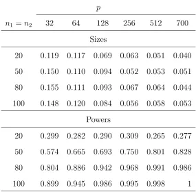
Table 3: Empirical sizes and powers of the proposed test for the variance-covariance matrices,
based on 1000 replications with Gamma distributed {Zijk} in Models (4.1) and (4.2).
p
n1 =n2 32 64 128 256 512 700
Sizes
20 0.119 0.117 0.069 0.063 0.051 0.040
50 0.150 0.110 0.094 0.052 0.053 0.051
80 0.155 0.111 0.093 0.067 0.064 0.044
100 0.148 0.120 0.084 0.056 0.058 0.053
Powers
20 0.299 0.282 0.290 0.309 0.265 0.277
50 0.574 0.665 0.693 0.750 0.801 0.828
80 0.804 0.886 0.942 0.968 0.991 0.986
100 0.899 0.945 0.986 0.995 0.998 1
second from
Xijk =Zijk+β1Zijk+1+· · ·+βm2Zijk+m2, (4.4)
for j = 1,· · · , n2, where the βi were chosen to be 0.8. We chose the lengths of the moving
averagem1andm2according to the dimensionpsuch that aspwas increased, the values ofm1
andm2were increased as well. Specifically, we set (m1, m2, p) = (2,25,50),(3,50,100),(7,100,200),(12,250
and (18,300,700) respectively. Two distributions were considered for the i.i.d. sequences
{Zijk}pk=1 in (4.3) and (4.4): (i) both sequences were standard normally distributed; (ii) the centralized Gamma(4,0.5) for Sample 1 and the centralized Gamma(0.5,√2) for Sample 2.
The simulation results for the second test are reported in Table 5 for the normally distributed
case and Table 6 for the Gamma distributed case.
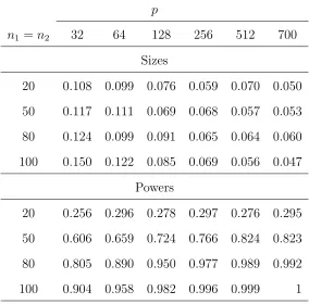
Table 4: Empirical sizes and powers of the proposed test for the variance-covariance matrices,
based on 1000 replications with the mixed normal and Gamma distributions for {Zijk} in
Models (4.1) and (4.2).
p
n1 =n2 32 64 128 256 512 700
Sizes
20 0.108 0.099 0.076 0.059 0.070 0.050
50 0.117 0.111 0.069 0.068 0.057 0.053
80 0.124 0.099 0.091 0.065 0.064 0.060
100 0.150 0.122 0.085 0.069 0.056 0.047
Powers
20 0.256 0.296 0.278 0.297 0.276 0.295
50 0.606 0.659 0.724 0.766 0.824 0.823
80 0.805 0.890 0.950 0.977 0.989 0.992
100 0.904 0.958 0.982 0.996 0.999 1
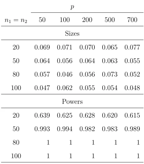
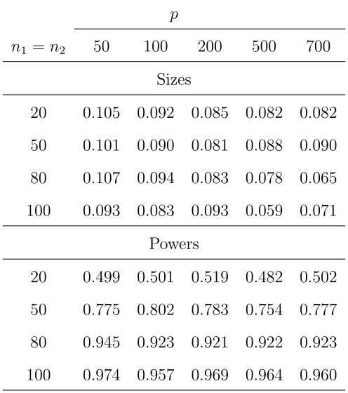
nominal 5% quite rapidly, while the powers were quite high and quickly increased to 1. For
the Gamma distributed case reported in Table 6, the convergence of the empirical sizes to the
nominal level was slower than the normally distributed case indicating that the convergence
of the asymptotic normality depends on the underlying distribution, as well as the sample
size and dimensionality. The powers in Table 6 were reasonable although they were smaller
than the corresponding normally distributed case in Table 5. Nevertheless , the power was
quite responsive to the increase of p and the sample sizes.
5. AN EMPIRICAL STUDY
We report an empirical study on a leukemia data by applying the proposed tests on the
Table 5: Empirical sizes and powers of the proposed test for the covariance between two
sub-vectors , based on 1000 replications for normally distributed{Zijk} in Models (4.3) and (4.4).
p
n1 =n2 50 100 200 500 700
Sizes
20 0.069 0.071 0.070 0.065 0.077
50 0.064 0.056 0.064 0.063 0.055
80 0.057 0.046 0.056 0.073 0.052
100 0.047 0.062 0.055 0.054 0.048
Powers
20 0.639 0.625 0.628 0.620 0.615
50 0.993 0.994 0.982 0.983 0.989
80 1 1 1 1 1
100 1 1 1 1 1
consist of microarray expressions of 128 patients with either T-cell or B-cell acute
lym-phoblastic leukemia (ALL); see Dudoit, Keles and van der Laan (2008) and Chen and Qin
(2010) for analysis on the same dataset. We considered a subset of the ALL data of 79
pa-tients with the B-cell ALL. We were interested in two types of the B-cell tumors: BCR/ABL,
one of the most frequent cytogenetic abnormalities in human leukemia, and NEG, the
cy-togenetically normal B-cell ALL. The number of patients with BCR/ABL was 37 and that
with NEG was 42.
A major motivation for developing the proposed test procedures for high-dimensional
variance-covariance matrices comes from the need to identify sets of genes which are
signif-icantly different with respect to two treatments in genetic research; see Barry, Nobel and
Table 6: Empirical sizes and powers of the proposed test for the covariances between two
sub-vectors, based on 1000 replications with Gamma distributed{Zijk} in Models (4.3) and (4.4).
p
n1 =n2 50 100 200 500 700
Sizes
20 0.105 0.092 0.085 0.082 0.082
50 0.101 0.090 0.081 0.088 0.090
80 0.107 0.094 0.083 0.078 0.065
100 0.093 0.083 0.093 0.059 0.071
Powers
20 0.499 0.501 0.519 0.482 0.502
50 0.775 0.802 0.783 0.754 0.777
80 0.945 0.923 0.921 0.922 0.923
100 0.974 0.957 0.969 0.964 0.960
and Reecy (2008) for comprehensive discussions. Biologically speaking, each gene does not
function individually, but rather tends to work with others to achieve certain biological tasks.
Gene-sets are technically defined vocabularies which produce names of gene-sets (also called
GO terms). There are three categories of Gene ontologies of interest: Biological Processes
(BP), Cellular Components (CC) and Molecular Functions (MF). For the ALL data, a
pre-liminary screening with gene-filtering left a total number of 2391 genes for analysis with 1599
unique GO terms in BP category, 290 in CC and 357 in MF.
Let us denote S1,· · ·,Sq forq gene-sets, whereSg consists ofpg genes. LetF1Sg andF2Sg
be the distribution functions corresponding toSg under the treatment and control, andµ1Sg
andµ2Sg be their respective means, and Σ1Sg and Σ2Sg be their respective variance-covariance
BP
P−values
Frequency
0.0 0.2 0.4 0.6 0.8 1.0
0
200
400
600
BP
L_n
Frequency
−2 0 2 4 6 8 10
0
100
200
300
CC
P−values
Frequency
0.0 0.2 0.4 0.6 0.8 1.0
0
50
100
150
CC
L_n
Frequency
−4 −2 0 2 4 6 8
0
10
30
50
MF
P−values
Frequency
0.0 0.2 0.4 0.6 0.8
0
50
100
150
MF
L_n
Frequency
−2 0 2 4 6
0
20
40
[image:24.612.151.448.79.375.2]60
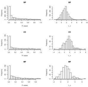
Figure 1: Histograms of P-values (left panels) for testing two covariance matrices and test
statistic Ln (right panels) for the three gene-categories.
the variance-covariance matrices. For the second hypothesis, we divided each gene-set into
two sub-vectors by selecting the first [p/2] dimensions of the gene-set as the first segment
and the rest as the second.
We first applied the proposed test for the equality of the entire variance-covariance
ma-trices and obtained the p-value for each gene-set. The p-values and the values of the test
statistics Ln as given in (2.7) are displayed in Figure 1 for the three gene-categories. By controlling the false discovery rate (FDR, Benjamini and Hochberg, 1995) at 0.05, 338 GO
terms were declared significant in the BP category, 77 in the CC and 75 in the MF, indicating
that the dependence structure among the gene-sets was significantly different between the
BCR/ABL and the NEG ALL patients for a large number of gene sets. That a relatively
surprising as we observe from Figure 1 that there were very large number of p-values which
[image:25.612.167.447.184.280.2]were very close to 0.
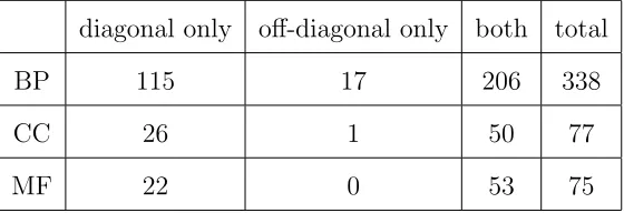
Table 7: Number of GO terms which were tested significantly different at the diagonal blocks,
off-diagonal blocks and both diagonal and off-diagonal blocks, respectively.
diagonal only off-diagonal only both total
BP 115 17 206 338
CC 26 1 50 77
MF 22 0 53 75
For those GO terms which had been declared having different variance-covariance
ma-trices, we carried out a follow-up analysis trying to gain more details on the differences by
partitioning the variance-covariance into four blocks in the form of (3.1) with p1 = [p/2]
and p2 = p−p1. We want to know if the difference was caused by the diagonal blocks or
the off-diagonal blocks. The tests on the two diagonal blocks were conducted using the first
proposed test for the variance-covariance matrix but with p1 orp2 dimensions, respectively.
The tests on the off-diagonal blocks were conducted by employing the second proposed test
for covariances between the two sub-vectors. The results are summarized in Table 7, which
provides the numbers of gene-sets which were tested significant in the diagonal matrices only,
the off-diagonal matrix only, and both at 5% . There were far more gene-sets which had
both diagonal and off-diagonal matrices being significantly different, and it was less likely
that the off-diagonal matrices were different while the diagonal matrices were otherwise. It
was a little surprising to see that the numbers of significant gene-sets for the diagonally-only,
off-diagonal only and both in each functional category added up to the total numbers exactly
for all three gene-categories.
As we have stated in the introduction, the proposed tests are part of the effort in testing
for high-dimensional distributions between two treatments. However, directly testing on
may endure low power. A realistic and intuitive way is to test for simpler characteristics
of the distributions, for instance testing for the means as in Bai and Saranadasa (1996)
and Chen and Qin (2010), and the variance-covariance as considered in this paper. For the
ALL data, in addition to testing for the variance-covariance, we also carried out tests for
the means proposed in Chen and Qin (2010) at a level of 5%. Table 8 contains two by
two classifications on the number and the probability of gene-sets which are rejected/not
rejected by the tests for the mean and the variance respectively. It is observed that it is far
more likely for the means to be significantly different than the variance-covariance, with the
probability of rejection being around 0.8 for the means versus 0.2 to 0.3 for the covariance
for the three functional categories. Given a gene-set which was not tested significant for
the means, the conditional probability of being tested significant for the covariance is lower
than that given a gene-set was not tested significant for the means. These were confirmed by
conducting the chi-square test for association for the three gene-set categories, which rejected
overwhelmingly (with p-values all less than 0.0005) the hypothesis of no-association between
being tested significant for the mean and the variance. For this particular dataset, the tests
for the means were quite effective in disclosing most of the differentially expressed
gene-sets. However, we do see that for Biological Processes and Cellular Component categories,
among those whose means were not declared significantly different, there were about 10% of
gene-sets having significant different covariance structures.
APPENDIX: TECHNICAL DETAILS.
As both Tn1,n2 and Sn1,n2 are invariant under the location transformation, we assumeµi = 0
throughout this section.
A.1. Derivations of Var(Tn1,n2) and Var(Sn1,n2)
tr{(Σ1−Σ2)2}. By noticing that Cov(An1, An2) = 0,
Var(Tn1,n2) = Var(An1) + Var(An2) + 4Var(Cn1n2)
− 4Cov(An1, Cn1n2)−4Cov(An2, Cn1n2). (A.1)
Adopting results from Chen, Zhang, and Zhong (2010), for h= 1 or 2,
Var(Anh) =
4 n2
h
tr2(Σ2h) + 8 nhtr(Σ
4
h) + 4∆h
nh tr(Γ
′
hΓhΓ′hΓh◦Γ′hΓhΓ′hΓh)
+ O{ 1 n3
h
tr2(Σ2h) + 1 n2
h
tr(Σ4h)}. (A.2)
Furthermore, we obtain
Var(Cn1n2) =
2 n1n2
tr2(Σ1Σ2) + (
2 n1
+ 2 n2
)tr(Σ1Σ2Σ1Σ2)
+ ∆1 n1
tr(Γ′
1Γ2Γ′2Γ1◦Γ′1Γ2Γ′2Γ1)
+ ∆2 n2
tr(Γ′2Γ1Γ′1Γ2◦Γ′2Γ1Γ′1Γ2) +o{
1 n1n2
tr2(Σ1Σ2)}
+ O
[
{√n1
1n2
+ 1 n1n2
+
2 ∑
i=1
(√1 ni +
1
ni)}Var(Cn1n2,1)
]
. (A.3)
By carrying out similar procedures, we are able to obtain Cov(An1, Cn1n2) and Cov(An2, Cn1n2).
After we substitute all the results into (A.1),
Var(Tn1n2) =
2 ∑ i=1 [ 4 n2 i
tr2(Σ2i) + 8 nitr(Σ
4
i) + 4∆i
ni tr(Γ
′
iΓiΓ
′
iΓi◦Γ
′
iΓiΓ
′
iΓi)
− 16n
i
tr(Σ2iΣ1Σ2)−
8∆i ni
tr(Γ′
iΣ1Γi◦Γ′iΣ2Γi) ]
+ 8
n1n2
tr2(Σ1Σ2) + (
8 n1
+ 8 n2
)tr(Σ1Σ2Σ1Σ2)
+ 4∆1 n1
tr(Γ′
1Γ2Γ′2Γ1◦Γ′1Γ2Γ′2Γ1) +
4∆2
n2
tr(Γ′
2Γ1Γ′1Γ2◦Γ′2Γ1Γ′1Γ2)
+ o{ 1 n1n2
tr2(Σ1Σ2)}+O [
{√n1
1n2
+ 1 n1n2
+
2 ∑
i=1
(√1 ni +
1
ni)}Var(Cn1n2,1) +
2 ∑
i=1
{n12
i
tr(Σ4i) + 1 n3
i
tr2(Σ2i)}
]
Similarly toTn1,n2, we have E(Sn1,n2) =tr{(Σ1,12−Σ2,12)(Σ1,12−Σ2,12)
′}and the leading
order terms in Var(Sn1n2) are given by
Var(Sn1n2) =
2 ∑
i=1 [
2 n2
i
tr2(Σi,12Σ′i,12) +
2 n2
i
tr(Σ2i,11)tr(Σ2i,22)
+ 4
nitr{(Σi,12Σ
′
1,12−Σi,12Σ′2,12)2}
+ 4
nitr{(Σi,11Σ1,12−Σi,11Σ2,12)(Σi,22Σ
′
1,12−Σi,22Σ′2,12)}
+ 4∆i ni tr{Γ
(1)
i
′
(Σ1,12−Σ2,12)Γ(2)i ◦Γ
(1)
i
′
(Σ1,12−Σ2,12)Γ(2)i }
]
+ 4
n1n2
tr2(Σ1,12Σ′2,12) +
4 n1n2
tr(Σ1,11Σ2,11)tr(Σ1,22Σ2,22). (A.5)
A.2. Proof of Theorem 1
The leading order terms in Var(Tn1,n2) are contributed by Anh,1 for h = 1,2 and Cn1n2,1,
which are defined by
Anh,1 =
1 nh(nh−1)
∑
i̸=j (X′
hiXhj)2, Cn1n2,1 =
1 n1n2
∑
ij (X′
1iX2j)2.
Hence, we only need to study the asymptotic normality ofZn1,n2 which is defined byZn1,n2 =:
An1,1+An2,1−2Cn1n2,1.
In order to construct a martingale sequence, it is convenient to have new random variables
Yi which are defined as
Yi = X1i for i= 1,2, ..., n1,
Yn1+j = X2j for j = 1,2, ..., n2.
To construct a martingale difference, we let F0 = {∅,Ω}, Fk = σ{Y1, ..., Yk} with k =
1,2, ..., n1 +n2. And let Ek(·) denote the conditional expectation given Fk. Define Dn,k =
(Ek−Ek−1)Zn1,n2 and it is easy to see that Zn1,n2 −E(Zn1,n2) =
∑n1+n2
k=1 Dn,k.
Proof. First of all, it is straightforward to show that EDn,k = 0. Next, by denoting
Sn,m =∑mk=1Dn,k = EmZn1,n2−EZn1,n2, we have Sn,q =Sn,m+ (EqZn1,n2−EmZn1,n2). Then
we can show that E(Sn,q|Fm) = Sn,m. This completes the proof of Lemma 1.
To apply martingale central limit theorem, we need Lemmas 2 and 3.
Lemma 2. Under Condition A2 and as min{n1, n2} → ∞, ∑n1+n2
k=1 σn,k2 Var(Zn1,n2)
p
− →1,
where σ2
n,k = Ek−1(Dn,k2 ).
Proof. To prove Lemma 2, firstly we can show E(∑n1+n2
k=1 σn,k2 ) = Var(Zn1,n2). Then we
will show that as min{n1, n2} → ∞, Var(∑kn1=1+n2σn,k2 )/Var2(Zn1,n2) → 0. To this end, we
decompose∑n1+n2
k=1 σ2n,k into the sum of eight parts, n∑1+n2
k=1
σ2n,k =R1+R2+R3+R4+R5+R6+R7+R8,
where with Q1,k−1 =∑ki=1−1(YiYi′−Σ1) and Q2,n1+l−1 =
∑l−1
i=1(Yn1+iY
′
n1+i−Σ2),
R1 =
n1
∑
k=1
8 n2
1(n1−1)2
tr(Q1,k−1Σ1Q1,k−1Σ1)
+ n2 ∑ l=1 8 n2
2(n2−1)2
tr(Q2,n1+l−1Σ2Q2,n1+l−1Σ2),
R2 =
n1
∑
k=1
16 n2
1(n1−1)
k−1 ∑
i=1
{Yi′(Σ31−Σ1Σ2Σ1)Yi},
R3 =
n2
∑
l=1
16 n2
2(n2−1)
[
tr(Q2,n1+l−1Σ
3
2)−tr{Q2,n1+l−1Σ2(
1 n1
n1
∑
i=1
YiYi′)Σ2} ]
,
R4 =
8 n2
1n2
n1
∑
i,j
tr(YjYj′Σ2YiYi′Σ2)−
16 n1n2
tr{Σ32( n1
∑
i=1
YiYi′)},
R5 =
n1
∑
k=1
4∆1
n2
1(n1−1)2
tr(Γ′
1Q1,k−1Γ1◦Γ′1Q1,k−1Γ1)
+ n2 ∑ l=1 4∆2 n2
2(n2−1)2
tr(Γ′2Q2,n1+l−1Γ2◦Γ
′
R6 = n1 ∑ k=1 8∆1 n2
1(n1−1)
tr{Γ′1(Σ1 −Σ2)Γ1◦Γ′1Q1,k−1Γ1},
R7 =
n2
∑
l=1
8∆2
n2
2(n2−1)
[
tr(Γ′
2Q2,n1+l−1Γ2◦Γ
′
2Σ2Γ2)
− tr{Γ′2Q2,n1+l−1Γ2◦Γ
′ 2( 1 n1 n1 ∑ i=1
YiYi′)Γ2} ]
and
R8 =
4∆2
n2 1n2
n1
∑
i,j
tr(Γ′2YiYi′Γ2◦Γ′2YjY
′
jΓ2)−
8∆2
n1n2
n1
∑
i=1
tr(Γ′2Σ2Γ2◦Γ′2YiY
′
iΓ2).
Therefore, we need to show that Var(Ri) = o{Var2(Zn1,n2)} for i= 1, ...,8.
For R1, there exists a constant K1 such that
Var(R1)≤K1{n1−4tr2(Σ21)tr(Σ41) +n−24tr2(Σ22)tr(Σ42)}.
Then, applying Var2(Zn1,n2)≥
16
n4 1tr
4(Σ2 1) + n164
2tr
4(Σ2
2) from (2.5), we know
Var(R1)
Var2(Zn1,n2) ≤ K161
{
tr(Σ4 1)
tr2(Σ2 1)
+ tr(Σ
4 2)
tr2(Σ2 2)
}
,
where tr(Σ4
1)/tr2(Σ21)→0 under Condition A2. Thus, Var(R1) =o{Var2(Zn1,n2)}.
By carrying out similar procedures we can show that the above is true for Ri with
i= 1, ...,8. Hence we complete the proof of Lemma 2.
Lemma 3. Under Condition A2, as min{n1, n2} → ∞ ∑n1+n2
k=1 E(Dn,k4 ) Var2(Zn1,n2)
→0.
Proof. For the case of 1≤k≤n1, there exists a constant csuch that
n1
∑
k=1
E(Dn,k4 )≤c
[
n−3
1 tr2{(Σ21−Σ1Σ2)2}+n−15tr4{(Σ21)} ]
.
Using the results Var2(Zn1,n2)≥64n
−2
1 tr2{(Σ21−Σ1Σ2)2}and Var2(Zn1,n2)≥16n
−4
1 tr4{(Σ21)}
from (2.5) and asn1 → ∞, we have ∑n1
k=1E(Dn,k4 ) Var2(Zn1,n2)
≤ c
n1 →
For the case of n1 < k < n1+n2, there exists a constantd such that
n∑1+n2
k=n1
E(D4n,k) ≤ d
n2 1n42
{2tr4(Σ1Σ2) +tr2(Σ1Σ2)tr2(Σ21)}
+ d
n1n42 [
2tr2(Σ
1Σ2)tr{(Σ22−Σ2Σ1)2} ]
+ d n5
2
tr4{(Σ2 2)}
+ d n4
2 [
2tr2(Σ2
2)tr{(Σ22−Σ2Σ1)2}+ 4tr2(Σ1Σ2)tr2(Σ22) ]
. (A.6)
To evaluate the ratio of individual term in (A.6) to Var2(Zn1,n2) respectively, we simply
replace Var2(Zn1,n2) by corresponding terms in (2.5). Then under Condition A2 and as
n2 → ∞, ∑nk=1+nn1+12 E(Dn,k4 )/Var2(Zn1,n2) → 0. Therefore, we complete the proof of Lemma
3.
With two sufficient conditions given in Lemmas 2 and 3, we conclude that
Zn1,n2 −E(Zn1,n2)
Var(Zn1,n2)
d
−
→N(0,1).
If we let ϵn1,n2 = An1,2 +An1,3 + An2,2 +An2,3 −2Cn1n1,2 −2Cn1n1,3 −2Cn1n1,4, then
Tn1,n2 =Zn1,n2 +ϵn1,n2. From Var(ϵn1,n2) = o(σ
2
n1,n2),
Var(ϵn1,n2
σn1,n2
) = Var(ϵn1,n2)
σ2
n1,n2
→0.
Moreover, E(ϵn1,n2) = 0. Therefore, ϵn1,n2/σn1,n2
p
−
→ 0. From Slutsky’s Theorem, we
complete the proof of Theorem 1.
A.3. Proof of Theorem 2
Recall that E(Anh) = tr(Σ 2
h) for h = 1 or 2. To show Anh/tr(Σ 2
h) p
−
→ 1, it is sufficient to
show that Var{Anh/tr(Σ 2
h)} →0.
From (A.2), we have
Var { Anh tr(Σ2 h) }
≤ tr2(Σ1 2
h)
[
4 n2
h
tr2(Σ2h) + 8 + 4∆h nh tr(Σ
4
h) +O{ 1 n3
h
tr2(Σ2h) + 1 n2
h
tr(Σ4h)}
]
,
where tr(Σ4
h)/tr2(Σ2h)→0 under Condition A2. Hence, Anh/tr(Σ 2
h) p
Moreover, under H0a : Σ1 = Σ2 = Σ, Anh/tr(Σ
2) −→p 1. Then using the continuous
mapping theorem, we have ˆσ0,n1,n2/σ0,n1,n2
p
− →1.
A.4. Proof of Theorem 3
The leading order terms in Var(Sn1,n2) are contributed byUnh,1andWn1n2,1 which are defined
by
Unh,1 =
1 nh(nh −1)
∑
i̸=j
Xhi(1)′Xhj(1)Xhj(2)′Xhi(2),
Wn1n2,1 =
1 n1n2
∑
ij
X1(1)i ′X2(1)j X2(2)j ′X1(2)i .
From Slutsky’s Theorem, we only need to study the asymptotic normality of Hn1,n2 which is
defined as Hn1,n2 =:Un1,1+Un2,1−2Wn1n2,1.
To implement martingale central limit theorem toHn1,n2, we need a martingale sequence.
To this end, we define random variables which are
Yi(1) = X1(1)i and Yi(2) =X1(2)i for i= 1,2, ..., n1,
Yn(1)1+j = X2(1)j and Yn(2)1+j =X2(2)j for j = 1,2, ..., n2.
If we define Cn,k = (Ek −Ek−1)Hn1,n2, where Ek(·) denote the conditional expectation
given Fk = σ{Y1, ..., Yk} with k = 1,2, ..., n1 +n2, we claim that {Cn,k,1 ≤ k ≤ n} is a
martingale difference sequence with respect to the σ-fields {Fk,1≤k ≤n} from Lemma 1.
We need Lemmas 4 and 5 to implement the martingale central limit theorem.
Lemma 4. Under Conditions A2 and A4, as min{n1, n2} → ∞, ∑n1+n2
k=1 τn,k2 Var(Hn1,n2)
p
− →1,
where τ2
n,k = Ek−1(Cn,k2 ).
Proof. First, we can show that E(∑n1+n2
k=1 τn,k2 ) = Var(Hn1,n2). Therefore, we only need
to show Var(∑n1+n2
k=1 τn,k2 ) = o{Var2(Hn1,n2)}to complete the proof of Lemma 4. To this end,
we decompose ∑n1+n2
k=1 τn,k2 into twelve parts, n∑1+n2
k=1
where with
O1,k−1 =
k−1 ∑
i=1
(Yi(1)Yi(2)′ −Σ1,12) and O2,n1+l−1 =
l−1 ∑
i=1
(Yn(1)1+iYn(2)1+i′ −Σ2,12),
P1 =
n1
∑
k=1
4 n2
1(n1−1)2
tr(O1,k−1Σ′1,12O1,k−1Σ′1,12)
+ n2 ∑ l=1 4 n2
2(n2−1)2
tr(O2,n1+l−1Σ
′
2,12O2,n1+l−1Σ
′
2,12),
P2 =
n1
∑
k=1
4 n2
1(n1−1)2
tr(O1,k−1Σ1,22O′1,k−1Σ1,11)
+ n2 ∑ l=1 4 n2
2(n2−1)2
tr(O2,n1+l−1Σ2,22O
′
2,n1+l−1Σ2,11),
P3 =
n1
∑
k=1
8 n2
1(n1−1)
tr{O1,k−1Σ′1,12(Σ1,12−Σ2,12)Σ′1,12},
P4 =
n1
∑
k=1
8 n2
1(n1−1)
tr{O1,k−1Σ1,22(Σ′1,12−Σ′2,12)Σ1,11},
P5 =
n2
∑
l=1
8 n2
2(n2−1)
tr{O2,n1+l−1Σ
′
2,12(Σ2,12−
1 n1
n1
∑
i=1
Yi(1)Yi(2)′)Σ′2,12},
P6 =
n2
∑
l=1
8 n2
2(n2−1)
tr{O2,n1+l−1Σ2,22(Σ
′
2,12−
1 n1
n1
∑
i=1
Yi(2)Yi(1)′)Σ2,11},
P7 =
4 n2
tr{(Σ2,12−
1 n1
n1
∑
i=1
Yi(1)Yi(2)′)Σ′2,12(Σ2,12−
1 n1
n1
∑
i=1
Yi(1)Yi(2)′)Σ′2,12},
P8 =
4 n2
tr{(Σ2,12−
1 n1
n1
∑
i=1
Yi(1)Yi(2)′)Σ2,22(Σ′2,12−
1 n1
n1
∑
i=1
Yi(2)Yi(1)′)Σ2,11},
P9 =
n1
∑
k=1
4∆1
n2
1(n1−1)2
tr(Γ(1)1 ′O1,k−1Γ(2)1 ◦Γ (1) 1
′
O1,k−1Γ(2)1 )
+ n2 ∑ l=1 4∆2 n2
2(n2−1)2
tr(Γ(1)2 ′O2,n1+l−1Γ
(2)
2 ◦Γ
(1) 2
′
O2,n1+l−1Γ
(2)
2 ),
P10 =
n1
∑
k=1
8∆1
n2
1(n1−1)
tr{Γ(1)1
′
(Σ1,12−Σ2,12)Γ(2)1 ◦Γ (1) 1
′
O1,k−1Γ(2)1 },
P11 =
n2
∑
l=1
8∆2
n2
2(n2−1)
tr{Γ(1)2 ′(Σ2,12−
n1
∑
i=1
Yi(1)Yi(2)′ n1
)Γ(2)2 ◦Γ(1)2 ′O2,n1+l−1Γ
(2)
P12 =
4∆2
n2
tr{Γ(1)2 ′(Σ2,12−
n1
∑
i=1
Yi(1)Yi(2)′ n1
)Γ(2)2 ◦Γ(1)2 ′(Σ2,12−
n1
∑
i=1
Yi(1)Yi(2)′ n1
)Γ(2)2 }.
For P1, there exists a constant J1 such that
Var(P1) ≤ 2 ∑ h=1 J1 n4 h
{tr2(Σh,12Σ′h,12)tr(Σh,11Σh,12Σh,22Σ′h,12)
+ tr(Σ2h,11)tr(Σ2h,22)tr(Σh,11Σh,12Σh,22Σ′h,12)
+ tr2(Σh,11Σh,12Σh,22Σ′h,12)}.
Using Var2(Hn1,n2)≥
8
n4
htr(Σ
2
h,11)tr(Σ2h,22)tr2(Σh,12Σ′h,12) from (3.8),
J1
n4
htr
2(Σh,
12Σ′h,12)tr(Σh,11Σh,12Σh,22Σ′h,12)
Var2(Hn1,n2)
≤ J1tr(Σh,11Σh,12Σh,22Σ
′
h,12)
8tr(Σ2
h,11)tr(Σ2h,22)
,
which goes to zero under condition A4 for h= 1 or 2.
Similarly, using Var2(Hn1,n2)≥
4
n4
htr
2(Σ2
h,11)tr2(Σ2h,22) from (3.8),
J1
n4
h
tr2(Σh,11Σh,12Σh,22Σ′h,12)/Var2(Hn1,n2)→0, and
J1
n4
h
tr(Σ2h,11)tr(Σ2h,22)tr(Σh,11Σh,12Σh,22Σ′h,12)/Var2(Hn1,n2)→0.
Hence, Var(P1) = o{Var2(Hn1,n2)}. Similarly, we have Var(Pi) = o{Var
2(Hn
1,n2)} for i =
1, ...,12. Therefore, we complete the proof of Lemma 4.
Lemma 5. Under Conditions A2 and A4, as min{n1, n2} → ∞ ∑n1+n2
k=1 E(Cn,k4 ) Var2(Hn1,n2)
→0.
Proof. For the case of 1≤k≤n1, there exists a constant csuch that
n1
∑
k=1
E(Cn,k4 ) ≤ c
[
n−13tr2{Σ1,11(Σ1,12−Σ2,12)Σ1,22(Σ′1,12−Σ
′
2,12)}
+ n−15tr2(Σ21,11)tr2(Σ21,22)
]
.
Applying Var2(Hn1,n2)≥16n
−2
1 tr2{Σ1,11(Σ1,12−Σ2,12)Σ1,22(Σ′1,12−Σ′2,12)}and Var2(Hn1,n2)≥
4n−14tr2(Σ21,11)tr2(Σ21,22) from (3.8) and asn1 → ∞, ∑n1
k=1E(Cn,k4 ) Var2(Hn1,n2)
≤ c
n1 →
For the case of n1 < k≤n1+n2, we can find a constantd such that
n∑1+n2
k=n1
E(C4
n,k)
≤ d
n3 1n32
tr(Σ1,11Σ2,11)tr(Σ1,22Σ2,22)tr(Σ22,11)tr(Σ22,22)
+ d
n3 2
tr2{(Σ2,11Σ2,12−Σ2,11Σ1,12)(Σ2,22Σ′2,12−Σ2,22Σ′1,12)}
+ d
n1n32
tr(Σ1,11Σ2,11)tr(Σ1,22Σ2,22)
×tr{Σ2,11(Σ2,12−Σ1,12)Σ2,22(Σ′2,12−Σ′1,12)}
+ d
n2 1n32
tr2(Σ1,11Σ2,11)tr2(Σ1,22Σ2,22) +
d n5
2
tr2(Σ22,11)tr2(Σ22,22). (A.7)
To evaluate the ratio of individual term in (A.7) to Var2(Hn1,n2) respectively, we simply
re-place Var2(Hn1,n2) by corresponding terms in (3.8). Then we can show that
∑n1+n2
k=n1+1E(C
4
n,k)/Var2(Hn1,n2)→
0. Therefore, we complete the proof of Lemma 5.
With two sufficient conditions given in Lemma 4 and 5, we know that
Hn1,n2 −E(Hn1,n2)
Var(Hn1,n2)
d
−
→N(0,1).
If we let ϵn1,n2 = Un1,2 +Un1,3 +Un2,2 +Un2,3 −2Wn1n1,2 −2Wn1n1,3 −2Wn1n1,4, then
Sn1,n2 =Hn1,n2 +ϵn1,n2. From Var(ϵn1,n2) = o(σ
2
n1,n2),
Var(ϵn1,n2
σn1,n2
) = Var(ϵn1,n2)
σ2
n1,n2
→0.
Moreover, we know E(ϵn1,n2) = 0. Therefore,ϵn1,n2/σn1,n2
p
−
→0. From Slutsky’s Theorem,
we complete the proof of Theorem 3.
A.5. Proof of Theorem 4
Applying the trace inequality, we know that tr2(Σh,
12Σ′h,12)≤ tr(Σ2h,11)tr(Σ2h,22). Therefore,
to prove Theorem 4, we first consider the case wheretr2(Σ
h,12Σ′h,12) = O{tr(Σ2h,11)tr(Σ2h,22)}.
From Theorem 2, we can show that A(1)nh/tr(Σ 2
h,11)
p
−
→ 1 and A(2)nh/tr(Σ 2
h,22)
p
−
→ 1. Moreover,
from (A.3), there exists a constantd1 such that
Var{Cn(i1)n2/tr(Σ1,iiΣ2,ii)} ≤ d1(
1 n1
+ 1 n2