Munich Personal RePEc Archive
Measuring seaports’ productivity: A
Malmquist productivity index
decomposition approach
Halkos, George and Tzeremes, Nickolaos
University of Thessaly, Department of Economics
July 2012
Online at
https://mpra.ub.uni-muenchen.de/40174/
!"
Department of Economics, University of Thessaly,
Korai 43, 38333, Volos, Greece
#
This paper uses three different Malmquist Productivity Index (MPI) decompositions to measure Greek seaports’ productivity for the time period 2006,2010. In addition bootstrap techniques are applied in order for confidence intervals of the MPIs and their components to be constructed and therefore to verify if the indicated changes are significant in a statistical sense. Finally, a second stage nonparametric analysis has been applied identifying the effect of seaports’ size on their productivity levels. The results reveal that the number of terminals is a crucial determinant of seaports’ productivity levels. In addition it appears that the high length of Greek seaports has a negative influence on their productivity levels over the years.
$ % Malmquist productivity index; bootstrap approach; nonparametric analysis; Greek seaports.
) *
Various research papers have been devoted to the examination of the
efficiency in the transport sector. Various approaches from simple performance
indicators to Total Factor Productivity (TFP), Stochastic Frontier Approach (SFA),
Data Envelopment Analysis (DEA) and Free Disposal Hull (FDH) models have been
used in every transport sector like public transit, railways, airports, airlines and
seaports. According to Gillen and Lall (1997), this growing interest has been
motivated by the need to investigate the results of deregulation, privatization and
commercialization.
Seaports play a significant role in the world trade and development (Tongzon,
2001). The assessment of seaport efficiency is of extreme importance because of the
increasing competition they face (Cullinane et al., 2006) which in turn creates the
need for better utilization of the available resources. Seaports are complex entities
which combine sea and land operations. Cullinane et al. (2002) identify two types of
ports, the comprehensive port which provides all the services and landlord port which
provides only the basic services. They have analyzed a port function matrix which is
an alternative way to distinct the types of seaports according to the services provided.
Econometric models, SFA and DEA have been used to assess the efficiency of
seaports. In their study, Roll and Hayuth (1993) apply a DEA model to measure the
efficiency of twenty seaports. Tongzon (2001) investigates the efficiency of sixteen
international seaports. The author utilizes a DEA model and uses land, labor, capital
and delay time as inputs and cargo and ship working rate as outputs. The later is used
as a measure of quality. Bonilla et al. (2002) employ DEA in order to measure the
commodities traffic efficiency of the seaports in Spain. Commodities traffic efficiency
DEA in Portuguese seaports and finds that the reform made by the authorities does
not fulfil the targets.
Similarly, Barros and Athanassiou (2004) compared the efficiency of seaports
in Portugal and Greece and provided benchmarks. They have used labor and capital as
inputs and ships, freight, cargo and containers as outputs. Cullinane et al. (2004) used
a DEA window analysis in order to achieve more robust results. Estache et al. (2004)
applied the Malmquist Productivity Index (MPI) to examine if seaport liberalization
was a success in Mexico. The results verify the success of the reforms made. Finally,
Cullinane et al. (2006) studied the top twenty ports in 2001 by using DEA and SFA.
Additionally they have used the SFA approach and found that the size of the port is
related to its efficiency levels. Manzano et al. (2008) employ an econometric model
and argue that efficiency tends to rise when the autonomy of seaport rises. Gonzales
and Trujillo (2008) apply a translog distance function in the top Spain seaports and
find that the reforms made in seaport industry had a positive effect on their
technological change.
In contrast to those studies our paper measures seaports productivity by
applying for the first time three different decompositions as has been introduced by
several authors (Färe et al., 1994a; 1994b; Ray and Desli, 1997; Gilbert and Wilson,
1998; Simar and Wilson, 1998a; Zofio and Lovell, 1998; Wheelock and Wilson,
1999). As well the inference approach introduced by Simar and Wislon (1999) is also
applied in order to construct confidence intervals for Malmquist productivity indices
and their decompositions. Finally, a second stage analysis is carried out by applying
nonparametric regression approaches aiming to establish how the size of the
The paper is structured as follows. Section two presents a brief literature of the
efficiency based studies and the different models applied to measure the efficiency
and productivity of transport units. Moreover, section 3 discusses the proposed
methodology, whereas section four presents the data and our empirical. Finally, the
last section concludes the paper.
+ ' %
In public transit industry, the government may consider two alternative
scenarios to reduce cost, such as privatization or the improvement of management
(Chu et al., 1992). Based on Hatry’s (1980) argument that efficiency and effectiveness
should be examined separately in public organizations, Chu et al. (1992) constructed
DEA models, one for efficiency and one for effectiveness, in order to assist public
agencies to monitor and improve their management. While efficiency refers to the
technical efficiency, effectiveness refers to the ability to use the outputs to fulfil the
managerial targets (Hatry, 1980). Chu et al. (1992) use various expenses as inputs and
vehicle hours of service as output for their efficiency model. For the effectiveness
model the authors use as inputs the output of the previous model along with some
exogenous variables such as population density and as outputs on their effectiveness
model they use the number of passenger trips.
Several studies apply DEA approach which is suitable for multiple input,
output cases. Chang and Kao (1992) study the efficiency of five bus firms in Taipei
using as inputs capital, labor and fuel and as outputs vehicle kilometers, revenue and
the number of bus trips. The authors find that private firms achieve better scores than
public,owned firms. Nolan (1996) and Karlaftis (2003) employ the same variables as
along with other variables by Kerstens (1996) who applies a DEA model at French
bus sector and finds that small firms have increasing while larger firms have
decreasing returns to scale.
Obeng (1994) by using labor, fuel and fleet size as inputs and vehicle miles as
output finds that technical efficiency decreases with the size of the firm. Viton (1998)
applies DEA and Malmquist productivity index to examine the efficiency of US bus
transit and finds that there is a slight improvement in productivity over time. Cowie
and Asenova (1999) examined the British bus sector after deregulation and
privatization and found high levels of inefficiency. Odeck (2008) applied a DEA and
Malmquist productivity index to examine the effect of mergers on the efficiency of
the Norwegian public bus sector finding evidence that mergers boost efficiency. In a
different study, Nozick et al. (1998) point out the problem of traffic congestion and
analyze a DEA model to investigate which travel demand management policy deals
with traffic congestion problem more effectively.
However, it must be emphasized that the majority of the studies in the
literature using various methodologies and approaches have concentrated in airline
industry. Oum and You (1998) used a translog variable cost function to assess the
competitiveness of the twenty two top airlines in the world, whereas Assaf (2009)
applied SFA investigating if US airlines are in crisis. The results indicate a decline in
efficiency scores. Schefczyk (1993) investigated the operational efficiency of fifteen
airlines using a DEA model and found that high operational performance is a leading
determinant of high profitability. Moreover, Peck et al. (1998) applied DEA to
examine the strategies of aircraft maintenance, whereas Capobianco and Fernandez
Scheraga (2004) examined the airline industry on the eve of the terrorist attack
of September 11th 2001. The author investigated thirty eight airlines around the globe
and concludes that the events had an effect not only on US airlines but also on other
major airlines. Moreover, Scheraga (2004) argues that airline carriers need to have
financial mobility in order to survive any unexpected event like a terrorist attack. The
author for the analysis has used a DEA model with available ton,kilometers, operating
costs and non,flight assets as inputs and revenue passenger and non,passenger
kilometers as outputs. Finally, Chiou and Chen (2006) applied a DEA model to
measure the cost efficiency, cost effectiveness and service effectiveness of fifteen
Taiwanese airlines.
Greer (2006) utilizes labor, fuels and seating capacity in a DEA model to
produce seat miles as the only output. The author investigates fourteen US airlines
and finds that low,cost carriers achieve better scores in technical efficiency. These
findings are verified by Barbot et al. (2008) for international airlines. Greer (2008,
2009) applies the same DEA model with Greer (2006) in US airlines. Greer (2008)
also utilizes a Malmquist productivity index and finds a significant improvement in
productivity over time. Greer (2009) uses a tobit regression in a second stage to study
the driver factors of efficiency. The findings indicate that average aircraft size,
average stage length and hubbing of the flights are significant factors while labor
unions are an insignificant factor. Barros and Peypoch (2009) in their study found that
demographics are an important factor for airline efficiency, while Quellette et al.
(2010) noted the significance of deregulation. Merkert and Hensher (2011) underline
the importance of aircraft size and the number of aircraft types on efficiency. They
argue that firms with large and few aircraft families achieve better efficiency scores in
A number of studies have also examined the efficiency of the airports which
are considered as a determinant factor for the economic development (Sarkis, 2000).
According to Adler and Berechman (2001) there are several factors an airline needs to
address in order to choose an airport including delays, runway capacity, costs and
traffic control. Parker (1999) examined the efficiency of British Aircraft Authority
before and after privatization and found that privatization had no impact on
efficiency. Parker (1999) used a DEA model with capital, labor, non,labor and capital
costs as inputs and passengers, cargo and mail as outputs.
Sarkis (2000) investigates the efficiency of forty four US airports by utilizing
a DEA model with operational costs, labor, gates and runaways as inputs and
operational revenue, passengers, cargo and general aviation movements as outputs.
He argues that hub airports and airports which are not in a snow belt are generally
more efficient. Adler and Golany (2001) developed a DEA model to determine which
airports are more likely to become the main gateway for airline companies.
Commenting on the DEA studies Adler and Berechman (2001) addressed the
importance of a quality variable in a DEA model for airports. Finally, Sarkis and
Talluri (2004) employed the same model with Sarkis (2000) and provided
benchmarks for inefficient airports whereas, Barros (2008) used SFA to investigate
the efficiency of Portuguese airports and reported that capital, prices, sales to planes,
sales to passengers and aeronautical fee are the main determinant factors of
,
Following Färe et al. (1994a) a multiple input and a multiple output at time
( )
- can be defined as:(
)
{
, : can produce}
, 1,...,= =
- (1)
where at time the input vector is indicated as =
(
1,...,)
∈ℜ+ and the outputvector is indicated as =
(
1,...,)
∈ℜ+. Then the output sets with respect tocan be defined as:
( )
={
:(
, ∈)
}
, =1,...,. - (2)
Additionally we assume that the output sets satisfy strong disposability, convexity and
they are bounded and closed.
Following Shephard (1970) production technology can be defined by an
output distance function as:
(
)
{
(
)
( )
}
(
)
( )
{
}
(
)
1, inf : / b , 1,...,
sup : / , 1,...,
ϕ
ϕ
ϕ
ϕ
−= ∈ =
= ∈ =
. .
(3)
where
ϕ
∈(
0,1]
and(
,)
≤1 if and only if(
.( )
)
. According to Färe et al.(1994b) the given inputs are defined as the maximum proportional expansion of the
outputs . The value of
(
,)
is given by / , where( )
{
( )
( )
}
Isoq : ,
ϕ
,ϕ
1∈ . = ∈. ∉. > and is the frontier output. If
(
,)
=1 then the production is technically efficient.In addition we need to define the distance function in different period and in
(
)
{
(
)
( )
}
1 1
, inf
ϕ
: /ϕ
, 1,...,+ = ∈ + =
.
(4)
According to Caves et al. (1982) the output oriented Malmquist productivity
index can be written as1:
(
1 1)
(
(
1,)
1)
, , ,
,
+ + + + =
(5)
The geometric mean of the Malmquist productivity index can be defined as:
(
)
{
(
)
(
)
}
(
)
(
)
(
(
)
)
1/ 2
1 1 1 1 1 1 1
1/ 2
1 1 1 1 1
1 , , , , , , , , , , , , , + + + + + + + + + + + + + = × = × (6)
(
1 1)
, , + , + can take the values >1(productivity growth), =1(stagnation) or
1
< (decline) between the periods and +1. As explained by Grosskopf (2003, p.
462) the Malmquist productivity index defined in (6) is linked to the average product
notion since the distance functions are calculated under the assumption of constant
returns to scale (CRS).
The initial decomposition of the index was provided by Färe et al. (1994a) as:
(
)
(
(
)
)
(
(
)
)
(
(
)
)
(
)
(
)
1/ 2
1 1 1 1 1
1 1
1 1 1 1
1 1 1 1
, , , , , , , , , , , , , , , + + + + + + + + + + + + + + + = × ×
= ΤΕ ×Τ
(7)
In equation (7) ‘ΤΕK’ measures technical efficiency change on the best practice
whereas ‘ΤK’ measures the geometric mean of the magnitude of technical change.
However the decomposition was made under the constant returns to scale (CRS)
1
assumption and best practice technologies may exhibit variable returns to scale (VRS)
technologies. Even though this decomposition is widely used by researchers to
measure productivity changes as suggested by Lovell (2003, p 443) this index
measures inappropriately productivity since their productivity change measure is
inappropriately defined on the best practice technologies, and in addition the scale
effect component is missing.
Therefore Färe et al. (1994b) redefined ΤΕ
(
, , +1, +1)
as:(
)
(
(
)
)
(
(
)
)
(
(
)
)
(
)
(
(
)
)
(
)
(
)
1 1 1 1 1 1 1 1 1
1 1
1 1 1 1 1
1 1 1 1
, , / , , , , , , / , , , , , , , , , , , , + + + + + + + + + + + + + + + + + + + +
ΤΕ = ×
= ΤΕ ×
= ΤΕ ×
(8)
As can be realized from (8) ΤΕ measures under the VRS assumption the technical
efficiency change whereas measures the change in scale efficiency between the
two periods. Therefore the Malmquist productivity index will take the form of:
(
)
(
)
(
)
(
)
1 1 1 1 1 1
1 1
, , , , , , , , ,
, , ,
+ + + + + +
+ +
= ΤΕ ×
×Τ
(9)
However Ray and Desli (1997) provided a different decomposition of Malmquist
productivity index2:
(
)
(
)
(
)
(
)
1 1 1 1 1 1
1 1
, , , , , , , , ,
, , ,
+ + + + + +
+ +
= ΤΕ ×
×Τ
(10)
where:
2
(
)
(
(
)
)
(
)
(
(
)
)
(
(
)
)
1 1 1 1 1
1/ 2 1 1
1 1
1 1 1 1
, , , , , , , , , , , , , + + + + + + + + + + + + +
ΤΕ =
Τ = ×
Then the ‘scale change factor was decomposed as:
(
)
(
)
(
)
(
)
(
)
(
(
)
)
(
(
)
)
(
)
(
)
(
(
)
)
1 1 1/ 21 1 1 1 1 1 1 1 1 1
1 1
1/ 2
1 1 1 1 1
1 , , , , / , , / , , / , , / , , , , , + + + + + + + + + + + + + + + + + + + + = × = × (11).
Finally, a third decomposition has been provided by several authors (Gilbert
and Wilson, 1998; Simar and Wilson, 1998a; Zofio and Lovell, 1998; Wheelock and
Wilson, 1999) defined as:
(
)
(
)
(
)
(
)
(
)
1 1 1 1 1 1
1 1 1 1
, , , , , , , , ,
, , , , , ,
+ + + + + +
+ + + +
= ΤΕ ×
×Τ × ΒΤ (12).
Whereas ΤΕ and ΤK are the same as Ray and Desli (1997) definition in (10). Moreover, is defined as Färe et al. (1994b) decomposition in (8) and the final
component ΒΤ is the scale bias of technical change and can be defined as:
(
)
(
(
)
)
(
(
)
)
(
)
(
)
(
)
(
)
1 1 1 1
1 1
1 1 1 1 1 1
1/ 2 1 1 , / , , , , , / , , / , , / , + + + + + + + + + + + + + +
ΒΤ =
× (13).
According to Lovell (2003, p.456) if scale efficiencies are different from the two
! ! " # "$
Having =1,..., seaports the frontier technology using data envelopment
analysis (DEA) methodology can be defined as:
(
)
{
}
, , 1 , , 1 ,, : 1,...,
1,..., 0 1,...,
ω
ω
ω
= = = ≤ = ≤ = ≥ =∑
∑
(14)where ω , indicates the intensity variable. In addition if
∑
ω
, =1 is added in (14) then the efficiency is calculated under the assumption of variable returns to scale. Asanalysed previously in order to calculate the Malmquist productivity index and its
components four distance functions are needed to be calculated for
(
,)
,(
)
1 1 1
,
+ + +
,
(
+1, +1)
and +1(
,)
following the linear programming as inFäre et al. (1994b).
Let
( )
′ be a seaport, and then the four output distance functions reciprocal to Farell’s (1957) output,based technical efficiency measurements can be calculated as:
(
)
(
)
1(
)
(
)
1, 1 , 1
, , , 1 1
, , , 1 1 , , max st 1,..., 1,..., 0 1,...,
ϕ
ω
ϕ
ω
ω
− ′ + ′ + ′ ′ ′ + = ′ + = = ≥ = = = ≥ =∑
∑
(16).As such the distances +1
(
,)
and +1(
+1, +1)
can be calculated accordinglyby changing +1 with and additionally the variable returns to scale can be imposed
by adding to the above linear programming problems the ,
1
ω
=∑
restriction.Moreover, according to Simar and Wilson (1998b, 1999, 2000a, 2000b) the
proposed bootstrap approach for constructing confidence interval for Malmquist
productivity indexes and their decompositions can be applied. The aim of the
following procedure is to estimate the population distribution of the Malmquist index
(component) and thus to make possible to test hypotheses regarding the true
parameter value (Hoff, 2006).
Letting %be the ‘true’ unknown index,
∧
%
be the DEA estimate of index as
indicated previously and * %,& to be the bootstrap estimates of the index as
calculated following Simar and Wilson (1999), then the basic assumption for
constructing the confidence intervals is that the distribution of
∧ −
% %
can be
approximated by the distribution of* ,
∧ −
% %
& . Therefore the values &α and
α
αcandefine the
(
1−α
)
confidence interval as:, ,
Pr
α
α 1α
∧ ≤ − ≤ = − % %
& (17)
and can be approximated from the bootstrap values α and αα
∧ ∧
*
, , ,
Pr
α
α 1α
∧ ∧ ∧ ≤ − ≤ = − % % &
& (18)
Then the bootstrap estimate of the
(
1−α
)
confidence interval for the th Malmqusit index or its component can be given by:,α ,
α
∧ ∧ ∧ ∧
− ≤ ≤ −
% % %
& (19)
In this way for the th seaport can be said that the Malmquist index (or/and its
component) is significantly different from unity at %α level if (19) does not include the value 1.
' (( ( )
Finally, a local linear estimator is applied in order to reveal the effect of
seaport size on their obtained Malmquist productivity index and its components.
Following Fan (1992, 1993) the local linear kernel model will have the form of:
(
* −)
+′ +
=
α
β
(20)given that can be seaport’s productivity measure (or its component) let* be the
variable(s) that determine seaport’s size, then by using the * − instead of
*
theintercept equals to
(
* =)
. If we fit the linear regression through the observations * − ≤' this can be written as:(
)
(
− − ′ * −)
%(
* − ≤')
∑
=1 2 ,min
α
β
β
α (21)
or setting
− = * 1
( )
( )
(
)
(
)
(
)
(
)
(
(
)
)
Κ −
Κ − ′
= − ≤ − ≤ ′ =
∑
∑
∑
∑
= − − = − = − = * + * + ' * % ' * % 1 1 1 1 1 1 1 1φ
φ
φ
φ
φ
φ
β
α
⌢ ⌢ (22)In equation (22) Κ
( )
. represents the kernel function and ' the bandwidth (or smoothing parameter) calculated by the least squares cross,validation data drivenmethod as suggested by Li and Racine (2004)3.
/ 0
Our analysis is applied on the main Greek seaports for the time period 2006,
2010 as has been reported by the Greek Seaport Authorities4. In addition for the
construction of output distance functions two inputs and two outputs has been used.
As described in table 1 the inputs used are total assets and number of employees and
the outputs are number of passengers travelled and tonnes of merchandise. Moreover
in order to examine how seaports’ sizes influence their productivity levels two
variables have been used as a proxy of seaport size (i.e. seaports’ length and the
number of terminals)5.
! # ) #
In addition to table1, table 2 provides the average values of the MPI and its
components following the three decompositions made over the examined time period.
Looking at the average values of productivity (MPI) over the years we can conclude
that only the time period of 2007,2008 the Greek seaports have been unproductive.
But it must be mentioned that MPI index records the average product notion since it is
3
The selection of bandwidth ' is very critical for our nonparametric regression analysis because when
∞ →
' (i.e. the smoothing is increased) the local linear estimator collapses to OLS regression of on * .
4
Access to statistics regarding the main Greek seaports can be obtained from: http://www.elime.gr/index.php/2011,09,16,07,14,33
5
All the data can be accessed from Eurostat at
measured under the assumption of constant returns to scale (equation 6). However as
has been suggested by Grosskopf (2003) the “true” underline technology can also
exhibit variable returns to scale.
! # ): Descriptive statistics of the variables
2006
2007
2008
2009
2010
Table 2 provides the 95% lower (LB) and upper (UB) confidence intervals
bounds as has been introduced by Simar and Wilson’s (1999) bootstrap methodology.
In addition table 2 provides seaports’ technical change under the assumption of
[image:17.595.64.503.210.640.2]the constant returns to scale hypothesis (ΤKCRS) has been used in the decomposition
provided by Färe et al. (1994a, 1994b) measuring the geometric mean of the
magnitudes of Greek seaports technical change along rays (equations 7,9) through
different periods (i.e. t+1 and t ).
As can be realized this measure does not correspond to the best practice
technologies therefore as Färe et al. (1994b) explained two other components must be
introduced. These are the technical efficiency change (ΤΕKVRS measured under best
practice technology) and the change in scale efficiency (SΕK). The results reveal that
during the periods 2007,2008 and 2008,2009 Greek seaports have increased technical
efficiency change (above 1) and decreased their scale efficiency change (i.e. below 1).
In addition when looking at the results for ΤKCRS we realize that seaports technical
progress has been improved during the period of 2007,2008. But it must be noted that
according to Lovell (2003) ΤKCRS does not capture correctly the shift in seaports’
frontier since it is calculated under the constant returns to scale.
Under the decomposition introduced by Ray and Desli (1997) seaports’
technical progress is measured correctly by the factor ΤKVRS. The results reveal that
Greek seaports have experienced technical progress under the periods 2006,2007 and
2009,2010 and not as reported by the ΤKCRS during the period 2007,2008. According
to Lovell (2003) and Grosskopf (2003) the MPI under the best practice technology is
the product of ΤKVRS and ΤΕKVRS.
In addition a component or a ‘residual’ component (Grosskopf, 2003, p.466) is
missing in order for the MPI under the VRS technology to be equal to the MPI given
by the ratio of average product (i.e. under the assumption of CRS,as in our case). This
component has been calculated by Ray and Desli (1997) and is the contribution of
having non,constant returns to scale (i.e. when SK >1). Therefore SK reflects the
contribution of scale economies on seaports’ productivity under the VRS technologies
between two periods (equation 11). Thus the results reveal a positive contribution of
scale economies to seaports’ productivity levels for the periods of 2006,2007, 2008,
2009 and 2009,2010.
! # +: Descriptive per period statistics of Malmquist index, components and 95% bootstrap confidence intervals
MPI ! Τ∆CRS ! Τ∆VRS ! ΤΕ∆VRS !
2006 2007
1.038 "#$%" &#&& 0.939 "#''( &#)*$ 1.069 "#(*+ &#+,& 0.912 "#)) &#"$( 0.314 "#)%( "#+&& 0.251 "#)+* "#%'+ 0.336 "#%"$ "#+$) 0.164 "#&*) "#)(, 0.672 "#**, "#',* 0.645 "#%'' "#(*) 0.592 "#+"+ "#,)( 0.517 "#&++ "#,)" 1.870 &#%"" )#)$$ 1.561 &#%+$ )#&'$ 1.661 &#+%( )#%+( 1.045 "#',( &#%+&
2007 2008
0.889 "#()+ "#$+$ 1.053 "#'*( &#*%( 0.886 "#+$$ &#)$% 1.015 "#"&* &#%'( 0.258 "#)*, "#)', 0.214 "#&,+ "#%)+ 0.122 "#"() "#)"+ 0.261 "#&(' "#%*" 0.451 "#+&' "#+*) 0.788 "#+)+ &#&+, 0.647 "#))( "#('* 0.416 "#&"$ "#*"* 1.497 &#+&' &#*+* 1.497 "#$%% )#)** 1.070 "#,)) &#'*) 1.622 "#("+ )#",'
2008 2009
1.019 "#$)" &#&"( 0.969 "#+"$ &#)&) 0.948 "#+"+ &#&*+ 1.054 "#,)) &#+*) 0.324 "#)'( "#++" 0.075 "#"%) "#&&& 0.086 "#"&& "#&+' 0.218 "#&+) "#%&+ 0.755 "#',, "#,*, 0.857 "#)($ &#"+% 0.825 "#)", "#$") 0.830 "#+(% &#&+" 1.836 &#+,) )#)'( 1.084 "#'&' &#+", 1.076 "#**) &#%,$ 1.677 &#%** )#%''
2009 2010
1.021 "#$*, &#"(" 0.865 "#*'& &#&+( 1.035 "#(%& &#%,& 0.977 "#+++ &#&'* 0.246 "#))* "#)'& 0.141 "#&%' "#)&& 0.149 "#"&$ "#)%& 0.122 "#&"& "#&(+ 0.546 "#*&* "#*$' 0.612 "#")& "#(+% 0.749 "#%(" "#$,) 0.663 "#&&' "#,*, 1.505 &#)(( &#'&( 1.172 &#")+ &#'*' 1.249 &#"+% &#'(* 1.205 "#''' &#*+$
SΕ∆ ! SΒΤ∆ ! S∆ ! 2006 2007
1.263 "#,($ &#'+, 0.919 "#*'% &#&&* 1.158 &#",& &#+)$ 0.354 "#)') "#*,, 0.170 "#"') "#&$" 0.338 "#%&, "#'$) 1.000 "#%"$ &#"') 0.520 "#"&$ "#''% 0.953 "#$)$ "#$(& 2.017 &#)&) )#(*) 1.198 &#"*" &#+%, 2.196 )#"(, %#*"&
2007 2008
0.871 "#%'$ &#&+" 1.172 "#*"* &#*** 0.954 "#(,, &#")) 0.215 "#&'& "#)+* 0.313 "#&$, "#'", 0.108 "#"%, "#&$* 0.442 "#)$) "#')& 0.898 "#*&" "#$%+ 0.765 "#%,* "#,(' 1.245 &#"&, &#*%' 2.083 "#$," %#&'( 1.118 &#"*, &#+%"
2008 2009
0.996 "#*)' &#)*) 1.024 "#',+ &#%"' 1.012 "#$*( &#&%, 0.211 "#&," "#%'' 0.084 "#"&" "#&$& 0.188 "#&') "#+)& 0.760 "#"'+ "#$(* 0.902 "#),* &#"+, 0.846 "#*%" "#$+' 1.61 "#$%" )#),, 1.182 "#$(% &#'++ 1.536 &#+)' )#%*'
2009 2010
Finally, a similar scale bias component (SΒΤK) has been introduced by several
authors (Gilbert and Wilson, 1998; Simar and Wilson, 1998a; Zofio and Lovell, 1998;
Wheelock and Wilson, 1999) and represents the changes of seaports’ scale
efficiencies between two periods (see equation 12,13). Therefore, if there are
differences between the scale efficiencies between two periods then seaports’
technical change (ΤKVRS) exhibits a scale bias. According to Lovell (2003, p. 456) it
measures the shift in seaports’ technical optimal scale between two period
technologies and can contribute to or detract from productivity growth. The results
reveal such contribution to seaports’ productivity growth for the periods 2007,2008
and 2008,2009.
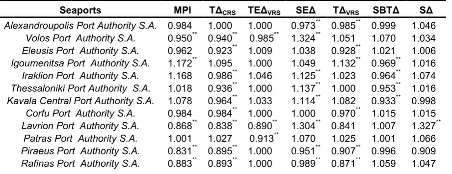
Table 3 provides the average values of MPI index and its components as has
been presented previously following the three decompositions. It also provides the
results obtained following the bootstrap procedure by Simar and Wilson (1999)
presented previously. Therefore, in the case of MPI it is reported that the seaport
Igoumenitsa Port Authority S.A. is productive over the years with an average
productivity of 1.172. The asterisks indicate that the value obtained is statistically
significant at 95% different from unity, following the bootstrap procedure presented
previously.
Furthermore, statistically significant differences from unity are reported for
the seaports of Volos Port Authority S.A., Lavrion Port Authority S.A., Piraeus Port
Authority S.A and Rafinas Port Authority S.A. However, as can be realised these
ports have reported to be unproductive over the time period of 2006,2010. In addition
all the rest of the seaports are reported to have statistically insignificant productivity
values at 95% indicating overall neutral productivity behaviour over the examined
decomposition reveals a statistical significant decline of Greek seaports technical
progress under the examined period.
More specifically the ports of Volos Port Authority S.A., Eleusis Port
Authority S.A., Iraklion Port Authority S.A., Thessaloniki Port Authority S.A.,
Kavala Central Port Authority S.A., Corfu Port Authority S.A., Lavrion Port
Authority S.A., Piraeus Port Authority S.A. and Rafinas Port Authority S.A. are
reported to have statistically significant ΤKCRS values below unity indicating that they
had a decrease on their technical change (under the assumption of CRS) over the
years. However, when we account for the best practice technologies (i.e. under the
assumption of VRS, ΤKVRS) the results reveal that five seaports have reported a
decline and one seaport an incline of their technical progress over the years.
Under the decompositions of Ray and Desli (1997) and several authors
(Gilbert and Wilson, 1998; Simar and Wilson, 1998a; Zofio and Lovell, 1998;
Wheelock and Wilson, 1999) the seaports with a decrease on their technical change
are Alexandroupolis Port Authority S.A., Eleusis Port Authority S.A., Corfu Port
Authority S.A., Piraeus Port Authority S.A. and Rafinas Port Authority S.A. But the
seaport of Igoumenitsa Port Authority S.A. is the only seaport reporting an increase
of its technical change over the examined period. Moreover, as it is reported three
seaports have decreased their technical efficiency change (ΤΕKVRS) over the years.
Under all the decompositions presented previously the seaports of Volos Port
Authority S.A., Lavrion Port Authority S.A. and Patras Port Authority S.A. have
decreased their technical efficiency change over the years, whereas the rest of the
seaports are reporting to have a stagnated technical efficiency change level.
Furthermore, under the decompositions of several authors (Färe et al., 1994b;
Wheelock and Wilson, 1999) five seaports have reported positive change on their
scale efficiency (SΕK) levels and three seaports a negative change. Following again
the bootstrap approach by Simar and Wilson (1999) the seaports with a positive scale
efficiency change are Volos Port Authority S.A., Iraklion Port Authority S.A.,
Thessaloniki Port Authority S.A., Kavala Central Port Authority S.A. and Lavrion
Port Authority S.A. Similarly the ports with the negative change on SΕK are
Alexandroupolis Port Authority S.A., Piraeus Port Authority S.A. and Rafinas Port
Authority S.A.
Moreover, the SΒΤK factor according to Lovell (2003) represents the scale
bias of seaports’ technical change over the years. It appears that four ports have
values below unity with 95% statistical significance, indicating that the shift in their
technically optimal scales has been detracted from their productivity growth. The
seaports with a reported scale bias are Igoumenitsa Port Authority S.A., Iraklion Port
Authority S.A., Thessaloniki Port Authority S.A. and Kavala Central Port Authority
S.A. Finally, under the decomposition provided by Ray and Desli (1997) the scale
change factor (SK) indicates that only in the case of Lavrion Port Authority S.A. a
statistically significant positive contribution (1.327) of seaport’s scale economies on
its productivity levels over the examined periods has been obtained. For all the other
seaports it appears that their scale economies have a neutral effect on their
productivity levels.
Following Li et al. (2009) we apply a test of equality density functions defined
over the MPI and its components between the examined periods. Additionally we
have bootstrap methods for obtaining the statistic's null distribution and the least
squares cross,validation method in order to smooth the MPI and its components as
distributions examined are equal, whereas under the alternative the two distributions
examined are not equal.
[image:23.595.86.547.180.357.2]! # ,: Average values of Malmquist productivity index and its decomposition components
Table 4 presents the results of the test obtained and the asterisks indicate the
bootstrap , obtained under 1%, 5% and 10% significance levels. As it appears
for the case of MPI we can realise that we cannot reject the null hypothesis of equality
of seaports’ MPI distributions over the years. The same result applies also for the
technical efficiency change (ΤΕKVRS), which indicates that seaports have the same
ΤΕKVRS distribution over the years. In addition with the results revealed previously
we can assume that over the years the policies’ imposed to the Greek seaports had
insignificant effect on their productivity and efficiency change levels.
In a similar manner it can be observed from the results presented in table 4
that few are the cases where the distributions are not equal between the examined
periods. For instance when looking at the ΤKVR we can realise that the distributions
are not equal between the periods of 2006,07 and 2007,08, also between the 2008,09
and 2009,10 and finally between 2007,08 and 2009,10, implying that seaports’
technical progress between those periods have changed. Similar results for rejecting Seaports MPI Τ∆CRS ΤΕ∆VRS SΕ∆ Τ∆VRS SΒΤ∆ S∆
- # #
. - # #
/ - # #
0 - # #
0 1 - # #
1 - # #
2 3 - # #
3 - # #
- # #
- - # #
- - # #
4 - # #
the null hypothesis at different statistical levels of significance are reported for some
cases of SK, SΒΤK, ΤKCRS and SEK.
! # /: Consistent density equality test for Malmquist productivity index and its components over the examined periods
MPI ΤΕ∆VRS
--.,-/ --/,-0 --0, - --.,-/ --/,-0 0,
--1,-. 0.212 0.670 0.040 --1,-. ,2.434 ,1.202 ,0.960
--.,-/ 0.167 0.170 --.,-/ 0.412 2.090
--/,-0 0.002 --/,-0 1.310
Τ∆CRS Τ∆VRS
--.,-/ --/,-0 --0, - --.,-/ --/,-0 0,
--1,-. 0.430 2.711* 0.696 --1,-. 1.056*** 1.749 0.412
--.,-/ 1.622 0.739* --.,-/ 1.252 1.059*
--/,-0 1.083* --/,-0 2.785***
SΕ∆ S∆
--.,-/ --/,-0 --0, - --.,-/ --/,-0 0,
--1,-. 0.195 ,0.357 ,0.959 --1,-. 2.724 1.870 4.547
--.,-/ ,0.196 0.926* --.,-/ ,1.252 2.376*
--/,-0 0.818* --/,-0 3.658*
SΒΤ∆
--.,-/ --/,-0 0,
--1,-. ,0.115* 1.708 ,0.249
--.,-/ 3.089 1.706
--/,-0 0.827*
666 9 : "#""&#; 66 9 : "#"*< 6 9 : "#&
Moreover, as presented previously we apply a local linear kernel regression in
order to see how the size of seaports affected their productivity levels and their
components. As a proxy of size we have used in our analysis two variables (seaport
length,PL and the number of terminals,NB). Figure 1 presents graphically the
combined effect6 of these two variables on the obtained productivity measures and its
components. As can be observed the effect of seaports’ length (PL) is negative on
6
1 ): The effects of seaports length (PL) and number of terminals (NB) on their productivity levels
1a 1b
1c 1d
1e 1f
their obtained productivity levels (i.e. when seaport’s length increases its productivity
decreases). The same effect appears also in the case of seaports’ technical progress
(both for CRS and VRS case), scale efficiency change, scale bias and for scale change
factor. However a positive effect of seaports’ length on its technical efficiency change
is observed.
Finally, when examining the effect of number of terminals on seaports’
productivity over the examined periods, a positive effect for MPI, ΤK (both for CRS
and VRS case) and for SΕK is recorded. As well it appears that seaports’ number of
terminals has a neutral effect on seaports’ SK and SBTK levels. At the same time, it is
observed that seaports’ terminal number has a negative effect on their technical
efficiency change over the years. As a general result we can interpret the findings that
number of terminals within a seaport is more important than seaport’s absolute length.
2 (
The paper contributes to the existing literature in two distinct ways. First and
in respect to methodologies applied, to our knowledge is the first study applying three
different decompositions of Malmquist productivity indexes as has been introduced
by several authors (Färe et al., 1994a; 1994b; Ray and Desli, 1997; Gilbert and
Wilson, 1998; Simar and Wilson, 1998a; Zofio and Lovell, 1998; Wheelock and
Wilson, 1999). In addition we apply the bootstrap approach (Simar and Wilson,
1999) on the obtained MPI and its components in order to verify if the indicated
changes are significant in a statistical sense or if there are products of sampling noise.
The second contribution of the paper lies on the application of a real case
study in the case of Greek seaports. The productivity and its components are
linear kernel model the effect of their sizes on the obtained productivity levels is
calculated. The results reveal that there are several productivity disparities among the
Greek seaports.
Under different decompositions it appears that the Greek seaports suffered
from stagnation of technological progress over the years. At the same time, the
empirical findings from these different decompositions indicate that Greek seaports’
scale effects have caused their productivity to decrease over the years. Finally, the
second stage nonparametric analysis revealed that Greek seaports’ length has a
negative effect on their productivity growth, whereas the number of terminals has a
positive effect.
3 4
Adler, N., Berechman, J., 2001. Measuring quality from the airlines’ viewpoint: an
application of data envelopment analysis. Transport Policy 8, 171,181.
Adler, N., Golany, B., 2001. Evaluation of deregulated airline network using data
envelopment analysis combined with principal component analysis with an
application to Western Europe. European Journal of Operational Research 132, 260,
273.
Assaf, A., 2009. Are US airlines really in crisis? Tourism Management 30, 916,921.
Barbot, C., Costa, A., Sochirca, E., 2008. Airlines performance in the new market
context: a comparative productivity and efficiency analysis. Journal of Air Transport
Management 14, 270,274.
Barros, C.P., 2003. Incentive regulation and efficiency of Portuguese port authorities.
Maritime Economics and Logistics 6, 55,69.
Barros, C.P., 2008. Technical change and productivity growth in airports: A case
study. Transportation Research Part A 42, 818,832.
Barros, C.P., Athanassiou, M., 2004. Efficiency in European seaports with DEA:
Evidence from Greece and Portugal. Maritime Economics and Logistics 6, 120,140.
Barros, C.P., Peypoch, N., 2009. An evaluation of European airlines’ operational
performance. International Journal of Production Economics 122, 525,533.
Bonilla, M., Medal, A., Casasus, T., Sala, R., 2002. The traffic in Spanish ports: An
efficiency analysis. International Journal of Economics Transport 29, 215,230.
Capobianco, H.M.P., Fernandez, E., 2004. Capital structure in the world airline
Chang, K., Kao, P., 1992. The relative efficiency of public versus private municipal
bus firms: an application of data envelopment analysis. Journal of Productivity
Analysis 3, 67,84.
Chiou, Y.C., Chen, Y.H., 2006. Route,based performance evaluation of Taiwanese
domestic airlines using data envelopment analysis. Transportation Research Part E 42,
116,127.
Chu, X., Fielding, G.J., Lamar, B.W. 1992. Measuring transit performance using data
envelopment analysis. Transportation Research Part A 26, 223,230.
Cowie, J., Asenova, D. 1999. Organization form, scale effects and efficiency in
British bus industry. Transportation 26, 231,248.
Cullinane, K., Song, D.W., Ji, P., Wang, T.F., 2004. An application of DEA windows
analysis to container port production efficiency. Review of Network Economics 3,
184,206.
Cullinane, K., Song, D.W., Gray, R., 2002. A stochastic frontier model of the
efficiency of major container terminals in Asia: assessing the influence of
administrative and ownership structures. Transportation Research Part A 36, 743,762.
Cullinane, K., Wang, T.F., Song, D.W., Ji, P. 2006. The technical efficiency of
container ports: Comparing data envelopment analysis and stochastic frontier
analysis. Transport Research Part A 40, 354,374.
Estache, A., Tavor de la Fe, B., Trujillo, L. 2004. Sources of efficiency gains in port
reform: a DEA decomposition of a Malmquist TFP index for Mexico. Utilities Policy
12, 221,230.
Fan, J., 1992. Design,adaptive nonparametric regression. Journal of the American
Fan, J., 1993. Local linear smoothers and their minimax efficiency. Annals of
Statistics 21, 196,216.
Färe, R., Grosskopf, S., Lindgren, B., Roos, P., 1994a. Productivity Developments in
Swedish Hospitals: A Malmquist Output Index Approach. In: Charnes, A., Cooper,
W.W., Lewin, A.Y., Seiford, L.M. (eds.), Data Envelopment Analysis: Theory,
Methodology and Applications, Kluwer Academic Publishers, Boston.
Färe, R., Grosskopf, S., Norris, M., Zhang, Z., 1994b. Productivity growth, technical
progress, and efficiency change in industrialized countries. American Economic
Review 84, 66,83.
Farrell, M., 1957. The measurement of productive efficiency. Journal of the Royal
Statistical Society Series A 120, 253,282.
Gilbert, R.A., Wilson, P.W., 1998. Effects of Deregulation on the Productivity of
Korean Banks. Journal of Economics and Business 50, 133–155.
Gillen, D., Lall, A., 1997. Developing measures of airport productivity and
performance: An application of data envelopment analysis. Transportation Research
Part E 33, 261,273.
Gonzalez, M.M., Trujillo, L., 2008. Reforms and infratrusture efficiency in Spain’s
container ports. Transportation Research Part A 42, 243,257.
Greer, M.R., 2006. Are the discount carriers actually more efficient than the legacy
carriers? A data envelopment analysis. International Journal of Transport Economics
33, 37,55.
Greer, M.R., 2009. Is it the labor unions’ fault? Dissecting the causes of the impaired
technical efficiencies of the legacy carriers in the United States. Transportation
Greer M.R. 2008. Nothing focuses the mind on productivity quite like the fear of
liquidation: Changes in airline productivity in the United States, 2000,2004.
Transportation Research Part A 42, 414,426.
Grosskopf, S., 2003. Some remarks on productivity and its decompositions. Journal of
Productivity Analysis 20, 459,474.
Hatry, H.P., 1980. Performance measurement principles and techniques: An overview
for local government. Public Productivity Review 4, 312,339.
Hayfield, T., Racine, J.S., 2008. Nonparametric Econometrics: The np Package.
Journal of Statistical Software 27, 1,32.
Hoff, A., 2006. Bootstrapping Malmquist Indices for Danish Seiners in the North Sea
and Skagerrak. Journal of Applied Statistics 33, 891,907.
Karlaftis, M.G., 2003. Investigating transit production and performance: a
programming approach. Transportation Research Part A 37, 225,240.
Kerstens, K., 1996. Technical efficiency measurement and explanation of French
urban transit companies. Transportation Research Part A 30, 431,452.
Li, Q., Maasoumi, E., Racine, J.S., 2009. A nonparametric test for equality of
distributions with mixed categorical and continuous data. Journal of Econometrics
148, 186,200.
Lovell, C.A.K., 2003. The decomposition of Malmquist productivity indexes. Journal
of Productivity Analysis 20, 437,458.
Manzano, J.I.C., Valpuesta, L.L., Perez, J.J., 2008. Economic analysis of the Spanish
port sector reform during the 1990s. Transportation Research Part A 42, 1056,1063.
Merkert, R., Hensher, D.A., 2011. The impact of strategic management and fleet
planning on airline efficiency: A random effects tobit model based on DEA efficiency
Nolan J.F., Ritchie, P.C., Rowcroft, J.E., 2001. Identifying and measuring public
policy goals: ISTEA and the US bus transit industry. Journal of Economic Behavior
and Organization 48, 291,304.
Nozick, L.K., Borderas, H., Meyburg, A.H., 1998. Evaluation of travel demand
measures and programs: A data envelopment analysis approach. Transportation
Research Part A 32, 331,343.
Obeng, K., 1994. Speciffication of long,run cost function to estimate input bias from
transit subsidies. Transportation Planning and Technology 18, 187,198.
Odeck, J., 2008. The effect of mergers on efficiency and productivity of public
transport services. Transportation Research Part A 42, 696,708.
Oum, T.H., You, C., 1998. Cost competitiveness of major airlines: an international
comparison. Transport Research Part A 32, 407,422.
Parker, D., 1999. The performance of BAA before and after privatization. Journal of
Transport Economics and Policy 33, 133,146.
Peck, M.W., Sheraga, C.A., Boisjoly, R.P. 1998. Assessing the relative efficiency of
aircraft maintenance technologies: an application of data envelopment analysis.
Transportation Research Part A 32, 261,269.
Quellette, P., Petit, P., Tessier Parent, L.P., Vigeant, S., 2010. Introducing regulation
in the measurement of efficiency, with an application to the Canadian air carriers
industry. European Journal of Operational Research 200, 216,226.
Ray, S.C., Desli, E., 1997. Productivity growth, technical progress, and efficiency
change in industrialized countries: Comment. American Economic Review 87, 1033,
1039.
Roll, Y., Hayuth, Y., 1993. Port performance comparison applying data envelopment
Sarkis, J., 2000. An analysis of the operational efficiency of major airports in the
United States. Journal of Operations Management 18, 335,351.
Sarkis, J., Talluri, S., 2004. Performance based clustering for benchmarking of US
airports. Transportation Research Part A 38, 329,346.
Schefczyk, M., 1993. Operational performance of airlines: an extension of traditional
measurement paradigms. Strategic Management Journal 14, 301,317.
Scheraga, C.A., 2004. Operational efficiency versus financial mobility in the global
airline industry: a data envelopment and tobit analysis. Transportation Research Part
A 38, 383,404.
Shephard, R.W., 1970. Theory of Cost and Production Functions. Princeton
University Press, Princeton, NJ.
Simar, L., Wilson, P.W., 1998a. Productivity Growth in Industrialized Countries
Discussion Paper 9810, Institut de Statistique, Universite Catholique de Louvain,
Louvain,la,Neuve, Belgium.
Simar, L., Wilson, P.W., 1998b. Sensitivity analysis of efficiency scores: how to
bootstrap in nonparametric frontier models. Management Science 44, 49–61.
Simar, L., Wilson, P.W., 1999. Estimating and bootstrapping Malmquist indices,
European Journal of Operational Research 115, 459,471.
Simar, L., Wilson, P.W., 2000a. A general methodology for Bootstrapping in
nonparametric frontier models, Journal of Applied Statistics 27, 779–802.
Simar, L., Wilson, P.W., 2000b. Statistical inference in nonparametric frontier
models: the state of the art. Journal of Productivity Analysis 13, 49–78.
Tongzon, J., 2001. Efficiency measurement of selected Australian and other
international ports using data envelopment analysis. Transportation Research Part A
Viton, P., 1998. Changes in multimode bus transit efficiency, 1988,1992.
Transportation 25, 1,21.
Wheelock D.C., Wilson, P.W., 1999. Technical progress, inefficiency, and
productivity change in U.S. banking, 1984–1993. Journal of Money, Credit, and
Banking 31, 212,234.
Zofio, J., Lovell, C.A.K., 1998. Yet Another Malmquist Productivity Index
Decomposition. Working Paper, Department of Economics, University of Georgia,