Multiple Threshold Effects for Temperature and Mortality

(1)

Munich Personal RePEc Archive

Multiple Threshold Effects for

Temperature and Mortality

Chen, Ping-Yu and Chen, Chi-Chung and Chang, Chia-Lin

Department of Applied Economics, Department of Applied

Economics, Department of Applied Economics and Department of

Finance National Chung Hsing University

21 November 2011

Online at

https://mpra.ub.uni-muenchen.de/35521/

(2)

Multiple Threshold Effects for Temperature and Mortality*

Ping-Yu Chen

Department of Applied Economics National Chung Hsing University

Email: [email protected]

Chi-Chung Chen**

Department of Applied Economics, National Chung-Hsing University

Email: [email protected]

Chia-Lin Chang

Department of Applied Economics Department of Finance National Chung Hsing University Email: [email protected]

December 2011

---

* The authors wish to thank Michael McAleer for helpful comments and suggestions. The second and third authors are most grateful for the financial support of National Science Council, Taiwan.

(3)

Multiple Threshold Effects for Temperature and Mortality

Abstract

Heat waves and cold fronts have become frequent of late, and have caused

serious disruptions around the world, especially in the mid- and high-latitudes. In future,

human beings are likely to face more serious, frequent and long-lasting extreme climate

events, with consequent greater damage to human life. This paper uses the multiple

panel threshold model to test whether there are threshold effects between temperature

and mortality, using a panel of 78 major cities in 22 OECD countries for 1990-2008.

From the empirical analysis, we find that the relationship between temperature and

mortality has three threshold effects, namely 15.21℉ (-9.33℃), 46.97℉ (8.32℃), and

87.53℉ (30.85℃). If the temperature is below 15.21℉ (-9.33℃), the magnitude of the

temperature effect below 15.21℉ (-9.33℃) is greater than the effect between 15.21℉

(-9.33₀C) and 46.97℉ (8.32₀C). When the temperature exceeds 87.53℉ (30.85℃),

higher temperature leads to higher mortality rate. Based on the estimated coefficients of

mean temperatures in four regimes, we separate 78 cities into five areas with latitudes

below 30°, 31°-40°, 41°-50°, and 61°-70°, and predict the impacts of future climate change

on mortality for 2021-2040, 2041-2060, and 2061-2100. In summer, climate is predicted

to increase mortality rates for 2021-2040, 2041-2060, and 2061-2100. For latitudes 41°

-50° and 51°-60°, the increased mortality rate is much larger than for other latitudes. In

winter, the increased magnitude induced by climate change is found to be greater than in

(4)

1. Introduction

According to the Intergovernmental Panel on Climate Change (hereafter IPCC)

report in 2007, the phenomenon of the sustained increase in global surface temperatures

cause a higher frequency of heat waves. This report also predicted that extreme weather

events will become more serious and frequent in the future. Schar et al. (2004) predicted

that in the late 21st Century, changes in extreme temperatures in Europe will increase

considerably and make summer mean temperatures higher and their variability greater.

Moreover, Clark et al. (2006) found that the maximum temperatures for June, July, and

August will become much warmer, and the higher number of extremely hot days will be

more significant than the mean temperatures for Europe, North and South America, and

East Asia. The expected greater intensity, frequency, and duration of heat waves will

occur in these areas, especially in the mid- and high-latitudes. Moreover, even slight

changes in mean climate or variability might increase the frequency of extreme weather

and have a significant impact on human health and safety.

In Europe, many have suffered from both heat waves and cold waves in recent

years. The European Heat Wave in 2003 resulted in the deaths of nearly 35,000 people,

while nearly 15,000 people died in France. Since then, heat waves and cold waves have

occurred more frequently, such as the European Heat Wave and Cold Wave in 2006, the

European Heat Wave in 2007, and the European Cold Wave in 2009-2010. In fact,

during the European Cold Wave in 2009-2010, UK experienced the coldest winter since

1963, with over 40,000 deaths. Not only Europe, but also North America, Australia and

Asia, have been unable to avoid heat waves and cold waves, such as the Northeast

United States Cold Wave in 2004, the North American Heart Wave in 2006, the Northern

Hemisphere Cold Wave in 2007, the Asian Heat Wave in 2007, the Australian Heat

Waves in 2008 and 2009, and the Japanese Heat Wave in 2010.

(5)

more appropriate in explaining mortality, and that average temperatures in summer and

winter have more significant influences on mortality than those in spring and autumn

(Ballester et al., 1997; Gemmell et al., 2000; Schwarts, 2005).

Some researchers have suggested that lower temperatures might have serious

negative impacts on human health (Bull and Morton, 1975; Diaz et al., 2002; Nicholls et

al., 2008; Loughna et al., 2010). However, Alfesio et al. (2002), Laaidi et al. (2006), and

Hajat et al. (2007) have suggested that not only decreases in winter temperatures, but

also increases in summer temperatures, would affect the mortality rate. In light of the

impact of unusual weather events on mortality, researchers have also concluded that

extreme temperatures, such as heat waves and cold waves, markedly increase mortality

(Baccini et al. 2008; Basu and Samet, 2003; Fouillet et al., 2006; Healy 2003; Johnson et

al., 2005; Keatinge et al. 1997; Keatinge et al., 2004; Kovats and Koppe, 2005;

McMichael et al., 2008; Montero et al., 2010; Nastos and Matzarakis, 2008; Rey et al.,

2009; Tobías et al., 2010; Vandentorren et al., 2004, 2006, 2008; Wenbiao et al., 2008).

Furthermore, outdoor workers, the elderly (65+ years), and the young (15- years) are at

high risk (Analitis et al., 2008; Basu et al., 2008; Chaudhury et al., 2000; Díaz et al.,

2005; Gouveia, 2003; Hajat et al., 2007; Ranhoff, 2000; Yip et al., 2008).

In addition, many researchers have attempted to determine the relationship between

mortality and temperature, which could be the V-, U- or J-shaped (Pan et al., 1995;

Huynen et al., 2001; Alfesio et al., 2002; Curriero et al., 2002; Kalkstein and Davis,

1989; McMichael et al., 2008, Armstrong, 2006; Laaidi et al., 2006). The V-, U- or

J-shapes show clear evidence of rising mortality with colder and hotter temperatures.

The estimated relationships between temperature and mortality could exhibit one or

more segments (or thresholds). Some studies have used other methods to estimate

temperature-mortality thresholds , such as the least total sum of squares (Kalkstein and

(6)

mortality is the lowest (EL-Zein et al., 2004), using a hockey stick (linear spline) model,

assuming a log-linear increase in risk below a cold threshold and above a heat threshold

(McMichael et al., 2008), the mortality anomaly, which is the deviation of the actual

death rate from the smoothed death rate (Nicholls et al., 2008; Loughnan et al., 2010),

and the 90th or 99th percentiles of temperature (Anderson and Bell, 2009).

The traditional approach determines the threshold level exogenously, which may

create some problems, such that we are unable to obtain confidence intervals for the

threshold level, and the estimates from the traditional approach may be sensitive to the

chosen threshold level (Hansen 1999, 2000). Hansen (1999) suggested the panel

threshold regression model to test for threshold effects and to search for two or more

regimes endogenously. This paper assumes there is an optimal average temperature, and

uses the panel threshold model to estimate average temperatures and the

mortality-temperature threshold. We use Hanson (1999)’s model to test whether there

exists a threshold effect between mortality and temperature, search for two or more

regimes endogenously, and then estimate the effects of different temperature regimes on

mortality.

For policy purposes, it is important to construct a reliable alert system for checking

extreme temperatures (high and low), which can trace temperatures effectively, and

predict heat waves and cold waves for increasing life safety and expectancy. In other

words, if a government knows in advance the critical temperature for heat waves, it

would be better prepared to avoid tragedies arising from heat waves. The empirical

findings in the paper should assist in determining how average temperatures can have

significant impacts on crude mortality rates, and thereby assist in public health policy.

The organization of the paper is as follows. In Section II, we discuss the data. In

Section III, we discuss the panel threshold regression model. The empirical results are

(7)

2. Data Description

The 78 major cities in 22 OECD countries in the sample were selected based on

availability of data (see Table 2). Monthly data for 1990-2008 were arranged in panel

data form. The crude mortality rate is the number of monthly deaths in each city divided

by the mid-month average total population of each city, and multiplied by 1,000, and are

obtained from the statistical bureaux in each country.

Real GDP per capita based on 2,000 US dollars is viewed as a measure of the

national economic development index. Data on real GDP and unemployment rate are

obtained from the OECD database. Mean temperatures and precipitation are obtained

from the International Research Institute for Climate and Society. We transform data on

daily average temperatures and dew points obtained from the National Climatic Data

Center into monthly temperature variations and mean dew points. The aforementioned

temperature indices are expressed in Fahrenheit.

The 22 OECD countries are Austria, Australia, Belgium, Canada, Switzerland,

Germany, Denmark, Spain, Finland, France, Greece, Hungary, Italy, Japan, Korea, the

Netherlands, Norway, Poland, Portugal, Sweden, the United Kingdom, and the United

States. The 78 major cities used in the paper are shown in the Appendix, with 42 cities

located in Europe and 36 cities located outside Europe.

The statistical descriptions for all the variables are shown in Table 1. The average

mortality rate for the 78 major cities in 22 OECD countries is 0.863, while mortality

ranges from 0.255 to 10.066. Table 1 also shows that the average GDP per capita in the

78 major cities is approximately US$ 2,941.53, which is higher than the global average.

The average unemployment rate for the 78 major cities in 22 OECD countries is 7.205%,

which is higher than that for developing countries. As economies become more highly

(8)

developing countries. The mean average temperature for the 78 major cities is 53.214℉,

with standard deviation 16.071. Mean precipitation is 68.386 mm, with standard

deviation 66.145, which means there are large changes in the 78 major cities for 22

OECD countries over time. The mean variance of temperatures is 36.778, with the range

of the variance of temperatures being 0.685 to 140.215.

3. Empirical Model

3.1 Single panel threshold model

This paper follows Hansen (1999)’s panel threshold model to examine whether the

mortality-temperature threshold exists for 78 major cities in the OECD. The structure of

the single panel threshold model follows Hansen (1999), as follows:

yit  i  xitI(qit  ) xitI(qit  )eit '

2 '

1   



 (1)

where the data are from a balanced panel, i and t denote indexes of the individual

(1iN) and time (1tT), respectively, yit and the threshold variable, qit, are

scalars, xit is a k vector of explanatory variables, I() is an indicator function, i is

the fixed effect (or heterogeneity of individuals), and the error term, eit, is assumed to

be independent and identically distributed, eit ~iid(0,2). Equation (1) can be written,

as follows:

it it

i

it x e

y  ' () ₍₂₎

where       ) ( ) ( ) ( _' 2 ' 1 ' r q I x r q I x x it it it it it _    .

The data are separated into two regimes, whereby the threshold variable, qit, is

less than or greater than the threshold value,  . The two regimes have different

regression slopes, ' 1

 and ' 2

 , respectively.

(9)

i i

i

it x e

y  ' () ₍₃₎

where





 T

t it i T y

y

1

/

1 ,





 T

t it i T x

x

1

/

1 , and





 T

t it i T e

e

1

/

1 .

Subtracting equation (3) from (2) leads to:

yit* 'xit*()eit* (4)

or, in vector form:

           * * 2 * iT i i y y y  ,

           ) ( ) ( ) ( * * 2 *    iT i i x x

x  , and

           * * 2 * iT i i e e e 

We stack the data over individuals into Y*, X*, and e*, and derive equation (5),

which is the model for estimating threshold effects:

           * * 1 * N y y Y  ,

           ) ( ) ( ) ( * * 1 *    N x x

X  , and

           * * 1 * N e e e  * ' *₍ ₎ * e X

Y    . (5)

Ordinary least squares (OLS) is used to estimate  for a given  :

()(X*()'X*())1X*()'Y*. (6)

The vector of regression residuals is:

*() * *()()

X Y

e   , (7)

which is minimized for SSE to estimate  :

( ) *( )' *( )

1  e  e 

SSE   (8)

where

 a r gm i n ₁()

 S S E

 

(9)

The estimated slope coefficient is (), the vector of residuals is e* e*(),

(10)

( ) ) 1 ( 1 ) ( ) ( ) 1 ( 1 1 * ' *'

2   

     SSE 

T N e

e T

N   

 . (10)

3.2 Multiple panel threshold model

Hansen (1999) extended the panel threshold model with more than one threshold,

as follows:

y_it  _i  x_itI(q_it  ) x_itI( q_it  ) 'x_itI(q_it  ₂)e_it

3 2 1 ' 2 1 '

1      



 (11)

where the threshold value, 1 ,is less than 2. Generally speaking, estimation of the

multiple threshold model is similar to the single threshold model. Three-stage estimation

is used for the two threshold parameters. The first stage for estimating the multiple

threshold model is the same as the single threshold model. SSE₁() is the single

threshold sum of squared errors, as defined in equation (8), and ˆ1 is the estimated

threshold parameter. Given the estimated threshold,ˆ₁, minimizing the SSE of equation

(11) estimates the second-stage threshold estimate, r 2

ˆ

 . The third stage is to re-estimate

the first-stage threshold, ₁, while the second-stage threshold estimate remains fixed,

thereby leading to asymptotically efficient estimators, r 1

ˆ

 and r 2

ˆ  .

Another difference is to determine the number of thresholds. If the F1 statistic

rejects the null hypothesis of no thresholds, a further test is required to distinguish

between one and two thresholds. The test is similar to the bootstrap procedure of the

single threshold model. In orer to minimize the second-stage SSE, ₂r(ˆ₂r)

SSE  , with the

residual variance estimate, ˆ 2(ˆ2)/ ( 1)

2 _ _

T N SSEr r

 , the likelihood ratio test of one

versus two thresholds is based on F2:

2 ( 1(ˆ1) 2(ˆ2))/ˆ2 r r

SSE SSE

F   . (12)

For constructing the confidence region of two estimated thresholds, ˆ1 and ˆ2,

the estimators have identical asymptotic distributions to the single threshold model (Bai,

(11)

threshold model:

2() ( 2(ˆ) 2(ˆ2))/ˆ2 r r r r SSE SSE

LR  

and

1() ( 1(ˆ) 1(ˆ1))/ˆ2 r r r r SSE SSE

LR   .

The asymptotic (1-α)% confidence intervals for ˆ2 and ˆ1 are the threshold

values,  , for LR2() c()

r _

and LR1() c()

r _

, respectively.

This paper presumes there is an optimal average temperature, and uses the panel

threshold model to investigate whether threshold effects exist between average

temperature and crude mortality rate. The empirical threshold model is as follows:

it it it it it it it it it it it it i it e unemp gdp temp dew prec temp I temp temp I temp temp I temp Mor               5 4 3 2 1 1 3 2 1 2 1 1 var ( )) ( ) (              (13)

for a balanced panel, where i is the index of city i for 22 OECD countries, and t is the

index of the time period (1990 to 2008). Morit represents monthly crude mortality rate,

it

pre represents monthly precipitation, dewit represents monthly average dew point

temperature, vartempit represents monthly variance of temperature, gdpit represents

monthly real gross domestic product per capita in 2000 US dollars, unempit represents

monthly unemployment rate, tempit is both an explanatory variable and the threshold

variable, which represents monthly average temperature, and  is the threshold value.

3.3 Testing for thresholds

It is necessary to test whether the estimated threshold effect is statistically

significant. The null hypothesis is H₀:₁ ₂ . Implementing the fixed-effect

transformation of equation (4) under the null hypothesis of no threshold effects, we

derive: ' * * 1 * ₍ ₎ it it

it x e

(12)

OLS is used to estimate the parameters, leading to the slope coefficient (~₁), the

residuals (e~it), and the sum of squared errors (

* *' 0 ~e ~e

SSE  ). The likelihood ratio test of

H0 is given by:

F₁ (SSE₀SSE₁(ˆ))/ˆ2. (15)

The unidentified threshold,  , under H0 leads to the problem of classical tests with

non-standard distribution. Hansen (1996) proposed using a bootstrap to estimate the

model under the null and alternative hypotheses, equations (4) and (14), respectively,

and computing the bootstrap value of the likelihood ratio test in equation (15). Repeating

this step and computing the percentage of simulated statistics beyond the actual value,

the asymptotic p-value of F1 under H0 may be found. If the p-value is less than the

critical value, the null hypothesis of no threshold effect is rejected.

After determining the existence of threshold effects, we test whether the estimated

ˆ is consistent with the true value, ₀. According to Chan (1993) and Hansen (1999),

when threshold effects exist, is consistent. However, there still exists the problem of

the non-standard asymptotic distribution. Hansen (1999) derived an optimal method for

the non-rejection region to test the threshold value,  , where the null hypothesis is

0 0 : 

H . The likelihood ratio test of  is given as follows:

1 ₂ 1

1 _ˆ

) ( )

( )

(



 

 S S E S S E 

LR   . (16)

Using specified assumptions (see Hansen, 1999, p.363), LR1()d , where  is

a random variable with asymptotic distribution and critical value given by:.

₎₎2

2 exp( 1 ( )

( x x

P      (17)

Based on Hansen (1999), the distribution function (17) can be written in equation

(18). Therefore, the non-rejection region for confidence level, 1, is the set of

(13)

c()2l o g (1 1). (18)

4. Empirical Results

This section presents the estimates for stationarity of the empirical model using

panel LM unit root tests, and tests whether there is a threshold relationship between

mortality and temperature, the number of mortality-temperature thresholds, and the

effects of climatic and macroeconomic factors on mortality. Finally, we combine the

estimated results of the panel threshold model and future climate data of the ECHAM5

model to predict how climate change influences mortality rate. This paper uses the

GAUSS9.0 software package to obtain the estimates of the panel LM unit root tests and

panel threshold models.

4.1 Panel LM unit root test

In order to avoid spurious regressions, all variables have to be stationary. We use

the panel LM tests (Im et al., (2005)) to test the stationarity of the six variables. If the

null hypothesis of the panel LM unit root test is rejected, all variables are stationary. The

results are reported in Table 2. Based on the outcomes of the LM panel unit root test

results with no break, one break, and two breaks, the LM unit root test with no break and

with one break support the non-stationarity of real GDP per capita and unemployment

rate, but the LM unit root test with two breaks supports the stationarity of all series at the

1% significance level. Hence, in the case of the panel LM unit root test with two breaks,

all series are stationary.

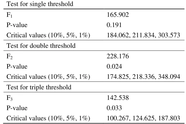
4.2 Testing for multiple thresholds

(14)

statistics of the thresholds. We examine sequentially the number of thresholds in the

model, and the threshold test results are given in Table 3. We can see the bootstrap

p-values of the single threshold are not significant. The test results of the double and

triple thresholds are significant at the 5% level, so there is strong evidence that triple

thresholds exist. Based on these results, we will use the triple threshold regression

model.

4.3 Panel threshold model results

The paper uses average temperature as the threshold variable to determine whether

the relationship between the average temperature and the mortality rate has a threshold

effect. We transform the data sets in the empirical model into logarithmic form to

capture the elasticity of mortality and climatic factors, and macroeconomic conditions.

Thus, a 1% variation in an individual factor, such as mean temperature, precipitation,

mean dew point temperature, real gdp per capita, and unemployment rate, induces a %

variation in the mortality rate.

Table 4 presents the three thresholds, their asymptotic 95% confidence intervals,

regression estimates, conventional OLS standard errors, and White standard errors. The

estimates are 15.21℉(-9.33℃), 46.97℉(8.32℃), and 87.53℉(30.85℃), that is,

temperature is separated into four regimes, namely very low temperature, low

temperature, moderate temperature, and very high temperature. Furthermore, the narrow

asymptotic confidence intervals for the threshold means there is little doubt about the

nature of the partition.

The four regression slopes in each of the four regimes are different. In the first

regime, if the average temperature is less than 15.21℉ (-9.33℃), a 1% increase in

average temperature results in 0.41% decrease in the mortality rate. In the second regime,

(15)

increase in average temperature results in 0.23% decrease in mortality rate. In the third

regime, if the average temperature ranges from 46.97℉ (8.32℃) to 87.53℉ (30.85℃), a

1% increase in the average temperature results in 0.074% increase in mortality rate. In

the last regime, if average temperature is greater than 87.53℉ (30.85℃), a 1% increase

in average temperature results in 0.30% increase in mortality rate.

The climate factors, namely the amount of precipitation, have significantly positive

effects on mortality rate, which is consistent with Ebi et al. (2004). The effects of

average dew point temperature on mortality rate are significantly positive, which is

similar to the finding in Guest et al. (1999). Temperature variation has a significant

positive effect on mortality rate, which is a similar to Applegate et al. (1981), Bull and

Morton (1975, 1978), Conti et al. (2005), Ellis et al. (1973), Ellis et al. (1980),

Greenberg et al. (1983), Jones et al. (1982), and Schwaetz (2000). In terms of

macroeconomic conditions, real GDP per capita has a significantly negative influence on

mortality rate, which indicates that higher income leads to lower mortality. Such

outcomes are consistent with the findings in Breault (1988), Buckley et al. (2004), Burr

(1997), Chung and Huang (2003), Gerdtham (2004), Gunnell et al. (2000), Huang and

Huang (1996), Mcleod et al. (2003), Neumayer (2003), and Smith (1999).

The unemployment rate influences mortality rate both significantly and positively,

which is similar to the findings in Brenner (1979, 1987), Brenner and Moonry (1983),

Platt (1984), and Stack (2000a, b). Although precipitation has a significant positive

impact on mortality using OLS standard errors, White’s standard errors suggest the

estimate is not significant.

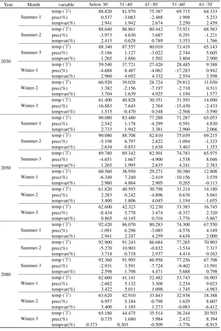
4.4 Impacts of future climate change on mortality

We integrate the estimated results of the panel threshold model with future climatic

(16)

taking the outputs of the ECHAM5 model for the A1B Scenario from IPCC’s Fourth

Assessment (2007). We separate the 78 cities into five areas with latitudes 30°, 31°-40°,

41°-50°, 51°-60°, and 61°-70°, and use the summer and winter months in three time slices

including 2021-2040 (denoted 2030), 2041-2060 (denoted 2050), and 2061-2100

(denoted 2080), to determine the influence of climate change, especially extreme

weather events, on mortality rate. Then we calculate the percentage change in monthly

total precipitation and monthly temperature variation relative to the baseline

(1990-2008), and monthly mean temperatures in 2030, 2050, and 2080 for the A1B

Scenario (see Table 5).

Combining the estimated results (Table 4) and the percentage changes in monthly

total precipitation and monthly temperature variations (Table 5), we evaluate the

changes in mortality rate caused by a 1% change in individual climate factors, namely

monthly total precipitation and monthly temperature variation. Regarding monthly mean

temperatures, we base the estimated coefficients of mean temperatures in the four

regimes to compute the impacts of relative changes between the 2030, 2050, and 2080

monthly mean temperatures and corresponding threshold temperatures on mortality

rates.

The effects of individual climatic factors and the composite impacts of climate

change on mortality rates in 2030, 2050, and 2080 for the A1B Scenario are given in

Table 6. In summer, future climate change increases the 2030, 2050, and 2080 mortality

rates. Especially, in latitudes 41°-50° and 51°-60°, the higher temperatures are much

larger than in other latitudes. In winter, the higher temperatures induced by climate

change are larger than in summer. Nevertheless, changes in mortality rates caused by

climate change gradually decrease. Especially for latitudes 41°-50°, 51°-60°, and 61°-70°,

the diminishing ranges are more remarkable than for other latitudes.

(17)

mortality rate in summer and winter are shown in Table 7 and Figures 1. The impacts of

summer climate change on mortality rate rise by degrees. Moreover, in 2080, the

increased mortality rate latitudes 41°-50° and 51°-60° exceed the same areas in winter.

Below latitude 30°, changes in mortality rate have a slightly increased trend. In latitude

61°-70°, the higher mortality rate is reduced in 2050, but is increased substantially in

2080.

5. Conclusion

This paper used Hansen’s (1999) multiple panel threshold model to estimate the

effect of climatic and macroeconomic factors on the mortality rate of 78 major cities in

22 OECD countries. We used average temperature as the threshold variable to determine

whether the relationship between average temperature and mortality rate involved

threshold effects.

The empirical results showed three thresholds, namely 15.21℉ (-9.33℃) , 46.97℉

(8.32℃), and 87.53℉ (30.85℃), when temperature was separated into four regimes,

namely very low temperature, low temperature, moderate temperature, and very high

temperature. In the very low temperature regime, average temperature was less than

15.21℉ (-9.33℃), a 1% increase in average temperature resulted in 0.41% decrease in

mortality rate. In the low temperature regime, average temperature ranged from 15.21℉

(-9.33℃) to 46.97℉(8.32℃), a 1% increase in average temperature resulted in 0.23

decrease in mortality rate. In the moderate temperature regime, average temperature

ranged from 46.97℉ (8.32℃) to 87.53℉ (30.85℃), a 1% increase in average

temperature resulted in 0.074% increase in mortality rate. In the very high temperature

regime, average temperature was greater than 87.53℉ (30.85℃), a 1% increase in

average temperature resulted in 0.30% increase in mortality rate.

(18)

variation are significantly positive on mortality rate. However, macroeconomic

conditions, namely real GDP per capita, have a significantly negative influence on

mortality rate, which indicates that higher income leads to lower mortality. On the other

hand, the unemployment rate has a significant and positive influence on mortality rate.

Finally, we integrated the estimates from the multiple panel threshold models with

future climate data to predict the impacts of future climate change on mortality for

2021-2040 (denoted 2030), 2041-2060 (denote 2050), and 2061-2100 (denoted 2080).

We separated 78 cities into five areas, with latitude below 30°, 31°-40°, 41°-50°, and 61°

-70°, and used summer and winter months in three time slices in 2030, 2050, and 2080 to

determine the influence of climate change especially extreme weather events, on

mortality rate. Based on the estimated coefficients of mean temperatures in four regimes,

we predicted the impacts of future climate change on mortality. In summer, future

climate is predicted to increase the 2030, 2050, and 2080 mortality rates. For latitudes

41°-50° and 51°-60°, the increased mortality rate is much larger than for other latitudes.

In winter, the increased magnitude induced by climate change is found to be greater than

in summer.

Extreme climate, whether cold or hot, has obvious significant influences on human

health. Using thresholds of the average temperatures on mortality rates to establish

policies, such as watch-warming systems, may help to prevent or mitigate the potential

(19)

Reference

Alfesio LF, Zanobetti A, Schwartz J: The effect of weather on respiratory and

cardiovascular deaths in 12 U.S. Cities.Environmental Health Perspectives 2002,

110: 859-863.

Analitis A, Katsouyanni K, Biggeri A, Baccini M, Forsberg B, Bisanti L, Kirchmayer U, Ballester F, Cadum E, Goodman PG, Hojs A, Sunyer J, Tiittanen P, Michelozzi P:

Effects of cold weather on mortality: results from 15 European cities within the

PHEWE project.American Journal of Epidemiology 2008, 168: 1397-1408.

Applegate WB, Runyan JW Jr, Brasfield L, Williams ML, Konigsbert C, Fouche C:

Analysis of the 1980 heat wave in Memphis.J Am Geriatr Soc 1981, 29: 337-42.

Armstrong B: Models for the relationship between ambient temperature and daily mortality.Epidemiology 2006, 17: 624-631.

Baccini M, Biggeri A, Accetta G, Kosatsky T, Katsouyanni K, Analitis A, Anderson HR, Bisanti L, D'Ippoliti D, Danova J, Forsberg B, Medina S, Paldy A, Rabczenko D, Schindler C, Michelozzi P: Heat Effects on Mortality in 15 European Cities.

Epidemiology 2008, 19: 711-719.

Bai J: Estimating multiple breaks one at a time. Econometric Theory 1997, 13: 315-352.

Ballester F, Corella D, Perez-Hoyos S, Saez M, Hervas A: Mortality as a function of

temperature. A study in Valencia, Spain, 1991-1993.Int J Epidemiol 1997, 26:

551-61.

Basu R, Feng WY, Ostro BD: Characterizing Temperature and Mortality in Nine California Counties. Epidemiology 2008, 19:138-145.

Basu R, Samet J: The relationship between elevated ambient temperature and

mortality: a review of the epidemiological evidence. Epidemiol Rev 2003,

24:190–202.

Breault K: Beyond the quick and dirty: reply to Girard. Am J Sociol 1988, 93: 1479–1486.

Brenner MH: Mortality and the national economy. A review, and the experience of

England and Wales, 1936-76.Lancet 1979, 2: 568-73.

(20)

Brenner MH, Mooney A: Unemployment and health in the context of economic change. Soc Sci Med 1983, 17: 1125-1138.

Buckley NJ, Denton FT, Robb AL, Spencer BG: The transition from good to poor health: an econometric study of the older population. J Health Econ 2004, 23: 1013-34.

Bull GM, Morton J: Relationships of temperature with death rates from all causes and from certain respiratory and arteriosclerotic diseases in different age

groups.Age Ageing 1975, 4: 232-246.

Bull GM, Morton J: Environment, temperature and death rates. Age Ageing 1978, 7: 210-24.

Burr JA, McCall PL, Powell-Griner E: Female labor force participation and suicide.

Soc Sci Med 1997, 44: 1847-59.

Chan KS: Consistency and limiting distribution of the least squares estimator of a continuous threshold autoregressive model. The Annals of Statistics 1993, 21: 520–33.

Chaudhury SK, Gore JM, Ray KCS: Impact of heat waves in India. Curr Sci 2000, 79:

153-155.

Chuang HL, Huang WC: Suicide and unemployment: is there a connection? An

empirical analysis of suicide rates in Taiwan. In 7th Annual Research Conference

on Economic Development, National Taipei University, Taipei, Taiwan; 2003.

Clark R, Brown S, Murphy, J: Modelling northern hemisphere summer heat extreme changes and their uncertainties using a physics ensemble of climate sensitivity

experiments.Journal of Climate 2006, 19: 4418-4435.

Conti S, Meli P, Minelli G, Solimini R, Toccaceli V, Vichi M, Beltrano C, Perini L:

Epidemiologic study of mortality during the summer 2003 heat waves in Italy.

Environ Res 2005, 98: 390-399.

Curriero FC, Heiner KS, Samet JM, Zeger SL, Strug SL, Patz JA: Temperature and

mortality in 11 cities of the Eastern United States. Am J Epidemiol 2002. 155:

80-87.

Díaz J, Garcı´a R, Lo´ pez C, Linares C, Tobı´as A, Prieto L: Mortality impact of

extreme winter temperatures. International Journal of Biometeorology 2005, 49:

(21)

Díaz J, García R, Velázquez de Castro F, Hernández E, López C, Otero A: Effects of extremely hot days on people older than 65 years in Seville (Spain) from 1986

to 1997.International Journal of Biometeorology 2002, 46: 145-149.

Ebi KL, Exuzides KA, Lau E, Kelsh M, Barnston A: Weather changes associated with hospitalizations for cardiovascular disease and stroke in California, 1983-1998.

Int J Biometeorol 2004, 49: 48-58.

Ellis FP, Princé HP, Lovatt G, Whittington RM: Mortality and morbidity in

Birmingham during the 1976 heat wave.Q J Med 1980, 49: 1-8.

El-Zein A, Tewtel-Salem M, Nehme G: A time-series analysis of mortality and air temperature in Greater Beirut.Sci Total_Environ_2004,₃₃₀_{: 71-80.}

Fouillet A, Rey G, Laurent F, Pavillon G, Bellec S, Guihenneuc-Jouyaux C, Clavel J, Jougla E, Hémon D: Excess mortality related to the August 2003 heat wave in France.Int Arch Occup Environ Health 2006, 80:16–24.

Gemmell I, McLoone P, Boddy FA, Dickinson GJ, Watt GC: Seasonal variation in mortality in Scotland.Int J Epidemiol 2000, 29: 274-279.

Gerdtham UG, Johannesson M: Absolute income, relative income, income inequality,

and mortality.J Hum Resou 2004, 22: 228-247.

Gouveia N, Hajat S, Armstrong B: Socioeconomic differentials in the

temperature-mortality relationship in Sao Paulo, Brazil. Int J Epidemiol 2003,

32:390-397.

Greenberg JH, Bromberg J, Reed CM, Gustafson TL, Beauchamp RA: The epidemiology of heat-related deaths, Texas – 1950, 1970-79, and 1980. Am J Public Health 1983, 73: 805-7.

Guest CS, Wilson K, Woodward A, Hennessy K, Kalkstein LS, Skinner C, McMichael AJ: Climate and mortality in Australia: retrospective study, 1979 – 1990, and predicted impacts in five major cities in 2030. Climate Res 1999, 13: 1-15.

Gunnell D, Shepherd M, Evans M: Are recent increases in deliberate self-harm associated with changes in socio-economic conditions? An ecological analysis of

patterns of deliberate self-harm in Bristol 1972-3 and 1995-6.Psychol Med 2000,

30: 1197-1203.

Hajat S, Kovats RS, Atkinson RW, Haines A: Impact of hot temperatures on deaths in

London: a time series approach. J Epidemiol Community Health 2002, 56:

(22)

Hajat S, Kovats RS, Lachowycz K: Heat-related and cold-related deaths in England and Wales: who is at risk?Occup Environ Med 2007, 64: 93-100.

Hansen BE: Inference when a nuisance parameter is not identified under the null hypothesis. Econometrica 1996, 64: 413–30.

Hansen BE: Threshold effects in non-dynamic panels: estimation, testing and inference.Journal of Econometrics 1999, 93: 345–68.

Hansen BE: Sample splitting and threshold estimation. Econometrica 2000, 68: 575-604.

Healy JD: Excess winter mortality in Europe: a cross country analysis identifying

key risk factors. Journal of Epidemiology and Community Health 2003, 57:

784-789.

Huang HL, WC Huang: A reexamination of sociological and economic theories of

suicide: a comparison of the U.S.A. and Taiwan.Soc Sci Med 1996, 43: 421-3.

Huynen MMTE, Martens P, Schram D, Weijenberg MP, Kunst AE: The impact of heat

waves and cold spells on mortality rates in the Dutch population.Environmental

Health Perspectives 2001, 109: 463-470.

Im KS, Lee J, Tieslau M: Panel LM unit root tests with level shift.Oxford B Econ Stat

2005, 67: 393-419.

IPCC (Intergovernmental Panel on Climate Change): Climate change 2007: the physical science basis. In: Solomon S, Qin D, Manning M, Chen Z and others (eds). Contribution of Working Group I to the Fourth Assessment Report of the Intergovernmental Panel on Climate Change. Cambridge University Press, Cambridge, 2007.

Johnson H, Kovats RS, McGregor GR, Stedman JR, Gibbs M, Walton H, Cook L, Black E: The impact of the 2003 heat wave on mortality and hospital admissions in England.Health Statistics Q 2005, 25: 6-12.

Jones TS, Liang AP, Kilbourne E, Griffin MR, Patriarca PA, Wassilak SG, Mullan RJ, Herrick RF, Donnell HD Jr, Choi K, Thacker SB: Morbidity and mortality associated with the July 1980 heat wave in St Louis and Kansas City, Mo.

JAMA 1982, 247: 3327-31.

Kalkstein LS, Davis RE: Weather and human mortality: an evaluation of

demographic and interregional responses in the United States. Ann Assoc Am

(23)

Keatinge WR, Donaldson GC, Bucher K, Jendritsky G, Cordioli E, Martinelli M, Dardanoni L, Katsouyanni K, Kunst AE, Mackenbach JP, McDonald C, Nayha S, Vuori I: Cold exposure and winter mortality from ischaemic heart disease, cerebrovascular disease, respiratory disease, and all causes in warm and cold

regions of Europe.The Lancet 1997, 349: 1341-1346.

Keatinge WR, Donaldson GC: The impact of global warming on health and

mortality. Southern Medical Journal 2004, 97: 1093-1099.

Kovats RS, Koppe C: Heatwaves: past and future impacts on health. In: Ebi KL, Smith J, Burton I (eds). Integration of Public Health with Adaptation to Climate Change: Lessons learned and New Directions. Lisse: Taylor & Francis Group, 2005, pp. 136–60.

Laaidi M, Laaidi K, Besancenot JP: Temperature-related mortality in France, a comparison between regions with different climates from the perspective of

global warming.International Journal of Biometerology 2006, 51: 145-153.

Loughnan M, Nicholls N, Tapper N: Mortality-temperature thresholds for ten major population centres in rural Victoria, Australia.Health Place 2010, 16: 1287-90.

Mcleod CB, Lavis JN, Mustard CA, Stoddart GL: Income inequality, household income, and health status in Canada: a prospective cohort study. Am J Public Health 2003, 93: 1287-93.

McMichael AJ, Wilkinson P, Kovats RS, Pattenden S, Hajat S, Armstrong B, Vajanapoom N, Niciu EM, Mahomed H, Kingkeow C, Kosnik M, O'Neill MS, Romieu I, Ramirez-Aguilar M, Barreto ML, Gouveia N, Nikiforov B: International study of temperature, heat and urban mortality: the 'ISOTHURM' project.

International Journal of Epidemiology 2008, 37: 1121-1131.

Montero JC, Miron IJ, Criado JJ, Linares C, Diaz J: Comparison between 2 methods

of defining heat waves: a retrospective study in Castile-La Mancha (Spain).Sci

Total Environ 2010, 408:1544–1550.

Nastos PT, Matzarakis AP: Variability of tropical days over Greece within the second half of the twentieth century. Theoretical and Applied Climatology 2008, 93: 75–89.

Neumayer E: Socioeconomic factors and suicide rates at large-unit aggregate levels:

a comment.Urban Stud 2003, 40: 2769-2776.

(24)

Australia.International Journal of Biometeorology 2008, 52: 375-384.

Pan WH, Li LA, Tsai MJ: Temperature extremes and mortality from coronary heart

disease and cerebral ingraction in elderly Chinese.Lancet 1995, 345: 353-355.

Platt S: Unemployment and suicidal behaviour: a review of the literature. Soc Sci Med 1984, 19: 93-115.

Ranhoff AH: Accidental hypothermia in the elderly. Int J Circumpolar Health 2000,

59: 255-259.

Rey G, Fouillet A, Bessemoulin P, Frayssinet P, Dufour A, Jougla E, Hémon D: Heat exposure and socio-economic vulnerability as synergistic factors in

heat-wave-related mortality.Eur J Epidemiol 2009, 24:495–502.

Schar C, Vidale PL, Luthi D, Frei C, Haberli C, Liniger MA, Appenzeller C: The role of

increasing temperature variability in European summer heatwaves. Nature

2004, 427: 332-336.

Schwartz J: The distributed lag between air pollution and daily deaths.

Epidemiology 2000, 11: 320-326.

Schwartz J: Who is sensitive to extremes of temperature? Epidemiology 2005, 16: 67-72.

Smith JP: Healthy bodies and thick wallets: the dual relation between health and economic status.J Econ Perspect 1999, 13: 144-66.

Stack S: Suicide: a 15-year review of the sociological literature. Part I: culture and economic factors. Suicide Life Threat Behav 2000, 30: 145-62.

Stack S: Suicide: a 15-year review of the sociological literature. Part II: modernization and social integration perspectives. Suicide Life Threat Behav

2000, 30: 163-76.

Tobías A, De Olalla P, Linares C, Bleda M, Caylà J, Díaz J: Short-term effects of extreme hot summer temperatures on total daily mortality in Barcelona, Spain.

InternationalJournalofBiometeorology 2010, 54: 115–117.

Vandentorren S, Bretin P, Zeghnoun A, Mandereau-Bruno L, Croisier A, Cochet C, Riberon J, Siberan I, Declercq B, Ledrans M: August heat wave in France: risk factors for death of elderly people living at home. European Journal of Public Health 2006, 16: 583–591.

(25)

Mortality in 13 French cities during the August 2003 heat wave. American Journal of Public Health 2004, 94: 1518–1520.

Vaneckova P, Hart MA, Beggs PJ, De Dear RJ: Synoptic analysis of heat- related

mortality in Sydney, Australia, 1993–2001. International Journal of

Biometeorology 2008, 52: 439–451.

Wenbiao H, Kerrie M, Anthony M, Shilu T: Temperature, air pollution and total

mortality during summers in Sydney, 1994–2004. International Journal of

Biometeorology 2008, 52: 689–696.

(26)

[image:26.595.88.516.148.376.2]

Figure 1. Impacts of summer and winter climate change on mortality rate

(27)

[image:27.595.90.524.115.327.2]

Table 1. Descriptive statistics for 22 OECD countries

Unit Mean Median Maximum Minimum Std. Dev.

Mortality % 0.863 0.744 10.066 0.255 0.691

GDP USD 2941.526 2656.437 13899.580 516.799 1431.144

Unemployment % 7.205 5.930 34.765 1.260 4.205

Temperature ℉

(℃)

53.214 (11.786)

54.600 (12.556)

96.500 (35.833)

0.003 (-17.776)

16.071 (9.640)

Precipitation Mm 68.386 51.600 1003.000 0.100 66.145

Variance of

Temperature

℉2

(℃)2

36.776 (10.998)

26.008 (8.389)

140.215 (57.844)

0.685 (0.558)

(28)

[image:28.595.89.532.116.326.2]

Table 2. Panel LM unit root test with no break, one break, and two breaks

Variables

With no break With one break With two breaks

LM statistic LM statistic LM statistic

Mortality rate -1.708** -1.963** -7.296***

Real GDP per capita -0.096 -0.952 -6.485***

Unemployment rate -0.423 -1.031 -6.362***

Average temperature -1.424* -1.776** -7.109***

Precipitation -1.409* -1.438* -7.220***

Dew point temperature -1.637** -2.079** -8.053***

Temperature variation -1.410* -2.035** -8.166***

Notes: *, **, and ***, respectively, denote significance at the 10%, 5%, and 1% level.

Table 3. Test for threshold effects

Test for single threshold

F1 165.902

P-value 0.191

Critical values (10%, 5%, 1%) 184.062, 211.834, 303.573 Test for double threshold

F2 228.176

P-value 0.024

Critical values (10%, 5%, 1%) 174.825, 218.336, 348.094 Test for triple threshold

F3 142.538

P-value 0.033

[image:28.595.139.465.448.666.2]

(29)

[image:29.595.99.507.108.535.2]

Table 4. Endogenous threshold regression for the triple threshold model

Threshold Estimates

Threshold Estimates 95% Confidence

Threshold1 15.206 [14.117, 15.328] Threshold2 46.973 [46.829, 47.215] Threshold3 87.526 [87.434, 87.660] Regime-dependent

Variable Coefficient OLS S.E. White S.E.

temp<15.206 -0.406*** 0.020 0.045

46.973>temp>15.206 -0.233*** 0.021 0.043

87.526>temp>46.973 0.074* 0.018 0.042

temp>87.526 0.295*** 0.017 0.042

Regime-independent

Variable Coefficient OLS S.E. White S.E.

Unemployment rate 0.287** 0.022 0.021

Real gdp per capita -0.973** 0.183 0.187

Temperature variation 0.488*** 0.062 0.103

Dew point temperature 0.029** 0.005 0.008

Precipitation 0.005* 0.001 0.002

Note: White denotes heteroscedasticity-consistent standard errors.

(30)

[image:30.595.79.534.68.750.2]

Table 5. Percentage change of future precipitation and temperature variation in 2030, 2050, and 2080 mean temperatures under the ECHAM5 model for A1B Scenario

Year Month variable below 30° 31°-40° 41°-50° 51°-60° 61°-70°

2030

Summer-1

temp (℉) 88.820 81.970 75.387 69.715 64.333 prec(%) 0.537 -3.083 -2.488 1.998 5.233 tempvar(%) 2.941 1.942 2.674 2.250 2.459

Summer-2

temp (℉) 88.640 86.861 80.442 73.921 68.563 prec(%) -3.973 4.630 3.687 0.291 -1.221 tempvar(%) 2.415 0.628 0.789 3.353 1.766

Summer-3

temp (℉) 88.340 87.557 80.010 73.419 65.143 prec(%) -5.186 1.127 -3.022 2.744 5.605 tempvar(%) 1.265 1.886 1.502 3.804 2.900

Winter-1

temp (℉) 59.540 37.721 27.428 28.485 9.388 prec(%) -4.688 8.487 -4.062 -17.283 0.942 tempvar(%) 2.960 4.692 4.332 2.554 3.598

Winter-2

temp (℉) 60.920 39.028 28.724 29.812 11.030 prec(%) 1.382 -2.156 -7.197 -2.710 0.511 tempvar(%) 3.704 1.639 4.925 1.194 1.577

Winter-3

temp (℉) 61.400 40.828 30.351 31.593 14.090 prec(%) -16.883 7.645 2.764 -15.430 -2.433 tempvar(%) 1.515 -0.470 0.348 -2.568 -3.590

2050

Summer-1

temp (℉) 90.080 83.480 77.288 71.287 65.053 prec(%) 2.542 1.178 -4.299 0.591 4.830 tempvar(%) 2.733 1.942 3.381 2.960 2.066

Summer-2

temp (℉) 90.080 88.708 82.810 75.039 69.215 prec(%) -5.198 6.797 2.822 -1.094 -1.333 tempvar(%) 2.634 0.853 1.638 3.463 1.353

Summer-3

temp (℉) 89.780 89.342 82.501 74.783 65.975 prec(%) -4.651 1.667 -4.900 1.538 8.046 tempvar(%) 1.265 1.995 2.635 4.241 2.383

Winter-1

temp (℉) 60.560 38.950 29.271 30.380 12.808 prec(%) -6.349 7.240 -2.419 -10.156 3.539 tempvar(%) 2.960 4.864 2.905 0.265 -0.113

Winter-2

temp (℉) 61.820 40.593 30.798 31.214 14.180 prec(%) 2.283 0.242 -4.896 0.670 5.041 tempvar(%) 3.400 1.806 4.045 1.194 -1.655

Winter-3

temp (℉) 62.600 42.323 32.230 33.383 16.745 prec(%) -8.434 5.778 3.474 -8.337 2.320 tempvar(%) 0.865 -0.145 0.316 -3.776 -5.867

2080

Summer-1

Summer-2

Summer-3

Winter-1

temp (℉) 62.660 41.141 32.482 33.743 16.903 prec(%) -2.682 5.132 3.308 2.234 9.023 tempvar(%) 3.422 5.011 1.098 -1.745 -4.983

Winter-2

temp (℉) 63.620 42.910 33.843 32.938 18.388 prec(%) 6.957 5.184 -0.798 1.629 8.607 tempvar(%) 3.400 1.185 1.273 -0.083 -6.412

Winter-3

(31)

[image:31.595.91.521.124.758.2]

Table 6. Impacts of mean temperature, precipitation, temperature changes on mortality rate under the ECHAM5 model for the A1B Scenario

Year Month variable below

30° 31°-40° 41°-50° 51°-60° 61°-70°

2030

Summer-1

temp 0.436 5.513 4.476 3.583 2.735 prec 0.003 -0.015 -0.012 0.010 0.026 tempvar 1.435 0.948 1.305 1.098 1.200 total 1.874 6.445 5.769 4.691 3.961

Summer-2

temp 0.375 6.284 5.273 4.245 3.401 prec -0.020 0.023 0.018 0.001 -0.006 tempvar 1.178 0.306 0.385 1.636 0.862 total 1.534 6.613 5.676 5.883 4.257

Summer-3

temp 0.274 0.011 5.204 4.166 2.862 prec -0.026 0.006 -0.015 0.014 0.028 tempvar 0.617 0.920 0.733 1.856 1.415 total 0.866 0.936 5.923 6.036 4.305

Winter-1

temp 1.980 4.589 9.695 9.170 15.535 prec -0.023 0.042 -0.020 -0.086 0.005 tempvar 1.444 2.290 2.114 1.246 1.756 total 3.401 6.922 11.789 10.330 17.296

Winter-2

temp 2.197 3.941 9.052 8.513 11.150 prec 0.007 -0.011 -0.036 -0.014 0.003 tempvar 1.807 0.800 2.404 0.583 0.770 total 4.011 4.730 11.420 9.082 11.922

Winter-3

temp 2.273 3.048 8.245 7.629 2.980 prec -0.084 0.038 0.014 -0.077 -0.012 tempvar 0.739 -0.229 0.170 -1.253 -1.752 total 2.928 2.857 8.428 6.299 1.216

2050

Summer-1

temp 0.861 5.751 4.776 3.830 2.848 prec 0.013 0.006 -0.021 0.003 0.024 tempvar 1.334 0.948 1.650 1.444 1.008 total 2.207 6.705 6.404 5.278 3.880

Summer-2

temp 0.861 0.398 5.646 4.421 3.504 prec -0.026 0.034 0.014 -0.005 -0.007 tempvar 1.286 0.416 0.799 1.690 0.660 total 2.120 0.848 6.459 6.106 4.157

Summer-3

(32)

Year Month variable below

30° 31°-40° 41°-50° 51°-60° 61°-70°

Winter-1

temp 2.140 3.980 8.781 8.231 6.404 prec -0.032 0.036 -0.012 -0.051 0.018 tempvar 1.444 2.374 1.418 0.129 -0.055 total 3.553 6.390 10.186 8.309 6.366

Winter-2

temp 2.339 3.165 8.023 7.817 2.739 prec 0.011 0.001 -0.024 0.003 0.025 tempvar 1.659 0.881 1.974 0.583 -0.808 total 4.010 4.047 9.973 8.403 1.957

Winter-3

temp 2.462 2.307 7.313 6.741 14.994 prec -0.042 0.029 0.017 -0.042 0.012 tempvar 0.422 -0.071 0.154 -1.843 -2.863 total 2.842 2.265 7.484 4.857 12.142

2080

Summer-1

Summer-2

Summer-3

Winter-1

temp 2.471 2.893 7.188 6.562 14.916 prec -0.013 0.026 0.017 0.011 0.045 tempvar 1.670 2.446 0.536 -0.851 -2.432 total 4.128 5.364 7.740 5.722 12.529

Winter-2

temp 2.623 2.016 6.513 6.962 14.179 prec 0.035 0.026 -0.004 0.008 0.043 tempvar 1.659 0.578 0.621 -0.040 -3.129 total 4.316 2.620 7.130 6.930 11.093

Winter-3

temp 2.868 1.239 5.684 5.322 13.130 prec 0.004 0.008 0.020 0.012 0.042 tempvar 0.182 0.148 -0.248 -1.843 -4.350 total 3.054 1.395 5.456 3.491 8.822

(33)

[image:33.595.117.494.125.246.2]

Table 7. Impacts of summer and winter climate change on mortality rate under the ECHAM5 model for the A1B Scenario

Season Year below 30° 31°-40° 41°-50° 51°-60° 61°-70°

summer

2030 4.274 13.995 17.367 16.610 12.523 2050 5.681 9.147 19.721 17.842 12.234 2080 9.561 11.347 23.438 20.954 11.848

winter

(34)

Appendix. The list of 78 major cities in 22 OECD countries

City Country City Country City Country

Sapporo Japan Krakow Poland Sydney Australia

Sendai Japan Gdansk Poland Darwin Australia

Tokyo Japan Oulu Finland Brisbane Australia

Nagoya Japan Helsinki Finland Adelaide Australia

Osaka Japan Vaasa Finland Hobart Australia

Hiroshima Japan Stockholm Sweden Melbourne Australia

Fukuoka Japan Malmo Sweden Boston USA

Edmonton Canada Umea Sweden St. Paul USA

Vancouver Canada Manchester UK Memphis USA

Winnipeg Canada London UK Kansas City USA

St. John's Canada Edinburgh UK Denver USA

Yellowknife Canada Berlin Germany Seattle USA

Toronto Canada Hamburg Germany Los Angeles USA

Montreal Canada Dusseldorf Germany Dallas USA

Whitehorse Canada München Germany Chicago USA

Seoul Korea Frankfurt Germany Washington USA

Zurich Switzerland Paris France Miami USA

Oslo Norway Nantes France New York USA

Trondheim Norway Lyon France

Tromso Norway Marseille France

Athens Greece Lisbon Portugal

Budapest Hungary Brussels Belgium

Roma Italy København Denmark

Palermo Italy Madrid Spain

Milano Italy Santander Spain

Groningen Netherlands Barcelona Sapin

Amsterdam Netherlands Valencia Sapin

Maastricht Netherlands Malaga Spain

Wien Austria Canberra Australia