Munich Personal RePEc Archive
On the finite-sample properties of
conditional empirical likelihood
estimators
Crudu, Federico and Sándor, Zsolt
University of Cagliari, CRENoS, Sapientia University, Miercurea
Ciuc
23 September 2011
ON THE FINITE-SAMPLE PROPERTIES OF
CONDITIONAL EMPIRICAL LIKELIHOOD
ESTIMATORS
Federico Crudu
yCRENoS, University of Cagliari
Zsolt Sándor
zSapientia University, Miercurea Ciuc
October 14, 2011
Abstract
We provide Monte Carlo evidence on the …nite sample behavior of the con-ditional empirical likelihood (CEL) estimator of Kitamura, Tripathi, and Ahn (2004) and the conditional Euclidean empirical likelihood (CEEL) estimator of Antoine, Bonnal, and Renault (2007) in the context of a heteroskedastic linear model with an endogenous regressor. We compare these estimators with three heteroskedasticity-consistent instrument-based estimators in terms of various per-formance measures. Our results suggest that the CEL and CEEL with …xed band-widths may su¤er from the no-moment problem, similarly to the unconditional generalized empirical likelihood estimators studied by Guggenberger (2008). We also study the CEL and CEEL estimators with automatic bandwidths selected through cross-validation. We do not …nd evidence that these su¤er from the no-moment problem. When the instruments are weak, we …nd CEL and CEEL to have …nite sample properties –in terms of mean squared error and coverage proba-bility of con…dence intervals– poorer than the heteroskedasticity-consistent Fuller (HFUL) estimator. In the strong instruments case the CEL and CEEL estimators with automatic bandwidths tend to outperform HFUL in terms of mean squared error, while the reverse holds in terms of the coverage probability, although the di¤erences in numerical performance are rather small.
Financial support from Marie Curie Excellence Grant MEXT-CT-2006-042471 is gratefully ac-knowledged.
y[email protected], University of Cagliari, Facoltà di Scienze Politiche, viale
Sant’Ignazio 78, 09123 Cagliari, Italy.
z[email protected], Sapientia University, Faculty of Economic and Human
1
Introduction
Motivated by the practical importance of models de…ned by conditional moment restric-tions, a number of recent important contributions have proposed empirical likelihood-based techniques for estimation and inference of this class of models. Kitamura, Tripathi, and Ahn (2004, KTA henceforth) develop a conditional empirical likelihood estimator of these models. Antoine, Bonnal, and Renault (2007, ABR henceforth) introduce an esti-mator based on a related idea that instead of the empirical likelihood uses the Euclidean likelihood. A common way of dealing with conditional moment restrictions is to reduce them to unconditional ones by means of instruments. However, this does not come without a cost, as it is generally di¢cult to …nd good instruments. The two estimators mentioned above are appealing from an asymptotic theoretical point of view as they are able to achieve semiparametric …rst-order asymptotic e¢ciency without computing the optimal instruments.
Smith (2007) generalizes the conditional empirical likelihood (CEL) of KTA and the conditional euclidean empirical likelihood (CEEL) of ABR to the class of local Cressie-Read discrepancies, where the termlocal refers to the explicit use of kernel weights. He shows that the estimators of the local Cressie-Read class are …rst order asymptotically equivalent to the CEL and CEEL (CE(E)L for short) estimators.
A few other recent contributions stress the potential of the conditional general-ized empirical likelihood (GEL) framework from an asymptotic theory point of view. Gospodinov and Otsu (2009) show that in an AR(1) model with iid errors the local GMM estimator, which is essentially the same as CEEL, has a higher order asymptotic bias smaller than the OLS estimator. Tripathi and Kitamura (2003) show that a test statistic for conditional moment restrictions based on the CEL objective function is asymptotically optimal in terms of a certain average power criterion.
the important class of models with endogenous regressors. Another problem that is important in practice is that, although the CE(E)L are instrument-free methods, they depend on additional unknown parameters, that is, bandwidths. The asymptotic the-ory of these estimators speci…es the rate at which the bandwidths should change with the sample size in order to obtain asymptotic e¢ciency, but this does not provide a clear indication on how to choose the bandwidths in practice. For some models (e.g., the linear heteroskedastic model in KTA, or the AR(1) model with ARCH errors in Gospodinov and Otsu, 2009) di¤erent bandwidth values lead to similar estimates. For models with endogenous regressors, however, it is not known to what extent the …nite sample performance of these estimators is a¤ected, if one uses di¤erent bandwidths, or if one uses some bandwidth selection procedure.
There are at least two reasons to expect CE(E)L to perform poorly in models with endogenous regressors, especially when the instruments are weak. First, these estima-tors are the result of a saddle point optimization problem, which may have extensive ‡at parts near the optimum. This may cause the distributions of these estimators to have no moments. Second, for a linear model with an endogenous regressor, Guggenberger (2008) …nds that the unconditional GEL estimators su¤er from the no-moment prob-lem. These estimators are also obtained as the outcome of a saddle point optimization problem, compared to which the dimensionality of the optimization problem increases considerably in the conditional moment case.
cri-terion proposed by Newey (1993). We then evaluate the performance of the estimators according to a range of criteria.
Due to their similarity to unconditional GEL estimators, the CE(E)L estimators may also su¤er from the no-moment problem. Therefore, interpretation of quadratic loss measures such as standard deviation and mean square error computed from Monte Carlo samples should be dealt with care. In order to avoid potential problems of in-terpretation, in addition to the standard measures of performance, we also look at performance measures like the median absolute error, the nine-decile range, and the tail probability, which do not depend on moments. Fiebig (1985) provides examples on how some estimators with no moments may be preferred to others that have moments. He suggests as a general evaluation criterion in this case the concentration of the estimator around the true parameter. In this respect, his probability of concentration criterion (Fiebig, 1985, equation (2)) is virtually the same as the tail probability statistic used in this paper and also in Guggenberger (2008).
Our results suggest that CEL and CEEL perform rather similarly. Both estimators computed with …xed bandwidths su¤er from the no-moment problem. We draw this conclusion from the fact that both estimators perform similarly to the HLIM estimator, which is known to have the no-moment problem (Hausman et al., 2010). We do not …nd evidence that the CE(E)L estimators with bandwidths computed by cross-validation have the no-moment problem. In addition, these estimators outperform their …xed bandwidth counterparts, especially in the weak instruments case. In this case, these estimators are outperformed by the HFUL estimator (Hausman et al., 2010), but in the strong instruments case they have competitive …nite sample properties with respect to the other estimators.
2
Monte Carlo experiment
In this section we describe the data generating process (DGP) in our Monte Carlo experiment and present the estimators that we study. For our DGP we consider a linear model with heteroskedastic errors that is similar to the one considered by Hausman et al. (2010). Speci…cally,
yi = 0xi+"i; i= 1; :::; n;
where xi is expected to be endogenous and the exogenous variable zi is observed. The parameter 0 is identi…ed by the conditional moment restriction
E(g(yi; xi; )jzi) = 0; (1)
where g(yi; xi; ) =yi xi. Regarding the primitives of our DGP we assume that
xi = zi+ui
where zi N(0;1),ui N(0;1), and
"i = ui+
s
1 2
2+:864 ( v1i+:86v2i)
withv1i N(0; z2i),v2i N(0; :862). The parameter is computed from the theoretical
R2 for the regression of "2
i onzi2, that is,
R2 = V ar(E("
2 i jz2i))
V ar(E("2
i jz2i)) +E(V ar("2i jz2i))
for given values of R2. This latter quantity measures the degree of heteroskedasticity, while determines the degree of endogeneity because corr(xi; "i) = =
p
(1 + 2). For
; R2 and we consider the following two parameter combinations:
; R2; = (0:75;0:1;1:863521);
; R2; = (0:30;0:2;1:38072):
degree of endogeneity accompanied by slightly more heteroskedasticity.1 We vary the
strength of instruments zi by taking = 0:4 and = 0:04; the latter value provides instruments with strength comparable to that in Guggenberger (2008), where in the case of one instrument the lowest correlation between the endogenous regressors and instruments is0:032. In order to see the e¤ect of the sample size on the performance of the estimators, we taken = 100and n= 200. Whenever we use estimators that require instruments, we consider the following two sets of 10and 30instruments:
zi = 1; zi; z2i; zi3; zi4; ziD1i; :::; ziD5i
0
(2)
zi = 1; zi; z2i; zi3; zi4; ziD1i; :::; ziD25i
0
;
where the variable Dki is a dummy variable that takes value 1 with probability 0:5. Similar dummies are used by Hausman et al. (2010).
In the next sections we describe the estimators that we consider.
2.1
Conditional empirical likelihood estimators
In this section we describe the CEL and CEEL estimators. These estimators are the result of a constrained optimization of certain nonparametric objective functions, where one of the constraints is the sample analog of the conditional moment restriction. The nonparametric objective functions are a nonparametric version of the log-likelihood func-tion for CEL, and a local quadratic Cressie-Read discrepancy criterion for CEEL, re-spectively (see KTA and ABR for further details, as well as Smith (2007) for a uni…ed treatment based on Cressie-Read discrepancy). In practice both estimators can be ob-tained from unconstrained optimizations of the so-called dual objective functions, which are derived from the …rst order conditions of the constrained optimization. These dual problems have the feature that they are saddle point optimization problems.
In particular, the CEL estimator of 0 is
bCEL= arg min max
i;i=1;:::;n
n
X
j=1 n
X
i=1
wijlog (1 + ig(yj; xj; )); (3)
1It would be desirable to study the case of high degree of heteroskedasticity as well. However, this
where wij, i; j = 1; :::; n are de…ned as
wij =
K zi zj
bn Pn
j=1K zi zj
bn
; (4)
that is, the weights of the Nadaraya-Watson nonparametric regression estimator, K is a density function onR, symmetric around 0, playing the role of a kernel function, and i; i= 1; :::; nare the Lagrange multipliers in the constrained maximization of the orig-inal objective function. Determining the CEL estimator from the dual (3) involves the …rst step maximization with respect to these Lagrange multipliers. A computationally e¢cient method for determining the Lagrange multipliers is discussed in the Appendix in Section B.1.
The CEEL estimator is
bCEEL = arg min
n
X
i=1
b
g( )2
Pn
j=1wijg(yj; xj; ) (g(yj; xj; ) bg( ))
!
; (5)
wherebgi( ) =Pnj=1wijg(yj; xj; )with weights given in (4). Di¤erently from the CEL estimator, the CEEL estimator does not require optimization with respect to the La-grange multipliers. This is because the quadratic Cressie-Read discrepancy criterion implies …rst-order conditions of the constrained optimization that allow for explicit ex-pressions of the Lagrange multipliers. Therefore, although not directly visible in the CEEL-objective function (5), CEEL estimation is also a saddle point problem. We also note that the CEEL estimator is numerically identical to a conditional generalization of the continuously updated GMM estimator of Hansen et al. (1996) (see ABR for further details).
The limiting distribution of the CE(E)L estimators is the same. That is, for k =
CEL; CEEL
p
n bk 0 !dN(0; V);
where
V = E D(z)2 (z) 1 1
The asymptotic variance of bk,k =CEL; CEEL, can be estimated as
b
Vk = n
X
i=1
b
D(zi)2 b bk; zi
1! 1
;
where b(zi); b bk; zi are nonparametric regression estimators of D(zi); bk; zi . Speci…cally, the Nadaraya-Watson nonparametric kernel regression estimators for our DGP are
b
D(zi) = n
X
j=1
wijxj;
and
b bCE(E)L; zi = n
X
j=1
wijg yj; xj;bCE(E)L 2
:
2.2
Instrumental variable estimation
Suppose that we have an L 1 vector of instrumental variables zi as described in (2). Then the conditional moment (1) implies the unconditional moment restrictions
E(zi(yi xi )) = 0;
which leads to estimation by means of GMM. GMM estimation generally requires a two step procedure. The …rst step estimator is given by the minimum of
QGM M( ) = (y x )0ZW Z0(y x )
for y and x being n 1 vectors of observations and Z is a n L matrix, such that its
ith row isz0
i. The resulting …rst step estimator is de…ned as
b1 = (x0ZW Z0x) 1x0ZW Z0y
for a certain positive de…nite matrixW. In our simulationsW is chosen to be the identity matrix. In order to achieve e¢ciency and robustness with respect to heteroskedasticity, in the second step we use an Eicker-White matrix (White, 1980):
where b =Pni=1 yi xib1 2
ziz0i. The GMM estimator is normally distributed
p
n bGM M !dN(0; VGM M)
and VGM M = (E(x0Z) 1E(Z0x)) 1
, for =E Z0(y x
0) (y x 0)
0
Z , which we estimate by VbGM M = x0Zb 1Z0x
1 .
In a recent paper Hausman et al. (2010) describe a simple one-step estimator that is robust to the presence of heteroskedasticity and many instruments. Such an estimator is similar to LIML and it is based on jackknife techniques. Let us …rst de…ne the projection matrix PZ = Z(Z0Z) 1Z0 and the diagonal matrix DPZ, whose diagonal elements are
the diagonal entries of PZ. Then, the so called HLIM estimator is computed as the minimum of
QHLIM( ) =
1 0A 1 1 0B 1 with
A = (y; x)0(PZ DPZ) (y; x); B = (y; x)
0
(y; x)
and is equal to
bHLIM = (x0(P
Z DPZ)x HLIMx
0x) 1(x0(P
Z DPZ)y HLIMx
0y) (6)
where HLIM is the minimum eigenvalue of the matrix B 1A. This estimator shares some features with LIML, most notably it may not have moments (Hausman et al. p. 8) in the weak instruments case. These authors propose a correction in the spirit of Fuller (1977), where the eigenvalue HLIM is replaced by
HF U L =
HLIM 1 HLIMn C
1 1 HLIM
n C
:
The parameterC is chosen by the econometrician and following the suggestion of Haus-man et al. (2010) we setC = 1. The so called HFUL estimator is then de…ned as
bHF U L = (x0(P
Z DPZ)x HF U Lx
0x) 1
(x0(P
Z DPZ)y HF U Lx
0y): (7)
Fork =HLIM; HF U L we have the following convergence in distribution:
bk 0 q
b
Vk
where
b
Vk=Mc 1SbMc 1; Mc=x0(PZ DPZ)x kx
0x and b S= n X i=1 _
x2i 2piixbix_i b"2i + L X t=1 L X s=1 n X i=1 e
ZitZeisb"i
! n X
j=1
ZjtZjsb"j
!
;
for, Ze = Z(Z0Z) 1
, b" = y xbk, bx = x b"x
0b"
b"0b", x_ = PZxb; furthermore, pii is the ith diagonal element of PZ. The limit of Vbk is provided in Hausman et al. (2010).
3
Implementation and results
We implement the CE(E)L estimators by using the Epanechnikov kernel:
K(u) = 3
4 1 u
2
1(juj 1);
where 1( ) is the indicator function. For the two sample sizes n = 100 and 200 we use the bandwidths bn in the sets
b100 2 f0:5;0:7;0:9;1:1;1:3;1:5;1:7;1:9g
and
b200 2 f0:3;0:5;0:7;0:9;1:1;1:3;1:5;1:7g:
As mentioned in the previous section, the CE(E)L estimators are the solution of a saddle point problem. Therefore, in certain situations that typically occur when the instruments are weak, the corresponding objective function may be very ‡at in the neighborhood of the optimum, causing the failure of standard optimization routines. In order to avoid this, we solve the optimization problem by means of a grid search. The grid we consider is between 25and 25and has step length 0:01.2 In order to provide
a fair comparison of performance, we also restrict the other estimates to the interval
[ 25;25]. We note that Guggenberger (2008) uses the same grid search approach in his study of unconditional GEL.
2This approach is not attractive from a computational point of view, in particular when the
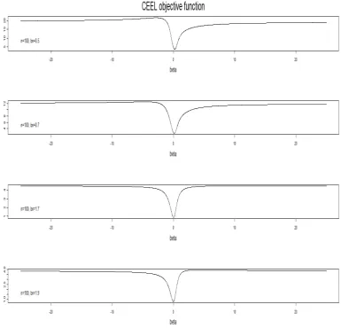
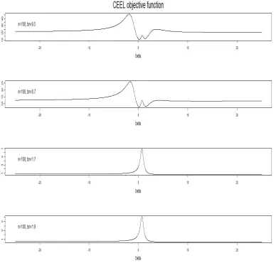
In order to provide some insight on the di¢culty of solving a saddle-point optimiza-tion problem, we make a few remarks on the behavior of the CE(E)L estimators for di¤erent bandwidths. First, in cases when the objective functions in (3) and (5) do not have ‡at parts around the optimum for any given bandwidth, the objective functions are similar, and, as a consequence, the estimates corresponding to di¤erent bandwidths will also be similar (the cases studied by KTA in their Monte Carlo experiments appear to be of this type). Second, whenever, for some bandwidths the objective function is ‡at near the optimum, the estimates corresponding to di¤erent bandwidths may be very di¤erent. We illustrate this phenomenon by plotting the objective function in these two cases.
Figure 1: CEEL objective function in the case of strong instruments and low endoge-nenity (R2 = 0:2; = 0:3 and = 0:4)
Figure 2: CEEL objective function in the case of weak instruments and high endoge-nenity (R2 = 0:1; = 0:75, and = 0:04)
using grid search instead of standard optimization routines such as Newton-Raphson or simplex search.
probability of a 95% con…dence interval (CovPr).3 The former provides us with
infor-mation on how spread out is the distribution of the estimator between the 5th and 95th percentile. The tail probability is computed as the relative frequency of the estimates for which b > 22:5 (we follow Guggenberger (2008) in choosing this number), and it conveys information on the fatness of the tails of the distribution of the estimators. The coverage probability of the symmetric95% con…dence interval is estimated by the relative frequency of the event b 0 1:96 b for a certain estimatorbof the true value 0, where bis an estimator of the standard error of b, which may di¤er across the various estimators we consider.
The focus of the Monte Carlo experiment is on the performance of the CE(E)L estimators in comparison with the instrument-based methods presented above. The latter may perform di¤erently if few or many instruments are included, speci…cally, in theory many instruments lead to asymptotic e¢ciency gains, but in practice they may lead to biased estimates. Therefore, for the three instrumental variable-based estimators we use two instrument sets ofL= 10and30instruments. Another objective in analyzing the results is to compare CEL to CEEL. CEEL has a computational advantage compared to CEL due to the fact that the Lagrange multipliers can be expressed explicitly and need not be estimated via numerical optimization as for CEL (see equations (3) and (5)).
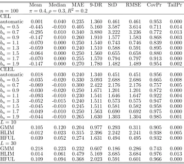
Before discussing the details with respect to the performance measures, we provide some general remarks. In none of the tables can we …nd an estimator that dominates all the others in the sense that it performs better with respect to all measures. The HLIM estimator is often similar to CE(E)L estimators with some …xed bandwidth, especially in the weak instruments case (Tables 1-2 and 5-6). The GMM estimator tends to perform well in terms of precision (MAE, StD), but performs poorly in terms of bias (Mean, Median) and coverage probability. HFUL has a rather sound performance compared to the other estimators in all the cases.
The two conditional empirical likelihood estimators, CEL and CEEL, have a rather
3Since Guggenberger (2008) uses similar simulation setup and performance measures for studying the
similar performance. Their performance is much better with automatic bandwidths than with …xed bandwidths in most of the cases. This is remarkable, because it contrasts the …ndings for a linear heteroskedastic model with an exogenous regressor, where CEL is only slightly better with automatic bandwidths than with …xed bandwidths (see KTA). This contrast is rather sharp in the weak instruments case. In what follows we make some distinctive comments on these and the strong instruments case, and then we discuss the properties of the estimators for each performance measure.
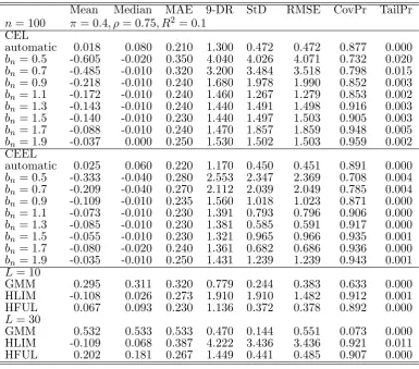
Weak instruments case (Tables 1-2 and 5-6). The CE(E)L estimators with …xed
bandwidths have large tail probabilities, similarly to the HLIM estimator, which is known to su¤er from the no-moment problem (Hausman et al., 2010). Therefore, the CE(E)L estimators with …xed bandwidths also have the no-moment problem in the weak instruments case. Besides the tail probabilities, these estimators perform rather poorly also with respect to the 9-DR.
The CE(E)L estimators with automatic bandwidths perform much better than their counterparts with …xed bandwidths. Their most remarkable feature is that they all have tail probabilities equal to0, which suggests that these estimators do not su¤er from the no-moment problem. In addition, their performance with respect to the two measures of dispersion MAE and 9-DR improves dramatically, although the latter values still remain high relative to those of GMM and HFUL. The same observation holds for the StD and RMSE. If we restrict the comparison to the criteria RMSE and CovPr, then HFUL (for both set of instruments) dominates CE(E)L in three out of the four tables, while in the fourth (Table 1) HFUL has just a slightly poorer CovPr. It is di¢cult to rank the CE(E)L and GMM even if we restrict the comparison to the criteria RMSE and CovPr, because in most cases GMM has lower RMSE but poorer CovPr.
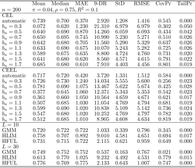
Strong instruments case (Tables 3-4 and 7-8). The CE(E)L estimators with
are rather competitive regarding the MAE, but poor regarding the RMSE, for several …xed bandwidth values. For n = 200 (Tables 7-8) CEEL works well for several …xed bandwidth values, while CEL is only slightly poorer with respect to the RMSE and CovPr.
The CE(E)L estimators with automatic bandwidths perform better than their coun-terparts with …xed bandwidths for n = 100 and rather similarly for n = 200. These estimators are rather competitive compared to the other estimators as well. A clear ranking is di¢cult to establish even if we restrict the comparison to RMSE and CovPr, but we can claim that CEEL has rather good CovPr and low RMSE in all four cases. Compared to HFUL, CEEL has similar CovPr and lower RMSE in almost all the cases.
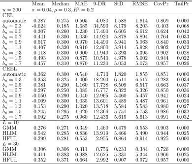
Mean bias. In the weak instruments case the CE(E)L have di¤erent bias values
for di¤erent bandwidths. The CE(E)L with automatic bandwidths have a performance comparable to the other estimators. The bias increases slightly for the GMM and HFUL estimators as the number of instrumentsL increases from10to30, while for the HLIM the change is ambiguous. In the strong instruments case, the CE(E)L are only biased for some very low …xed bandwidth values, while the CE(E)L with automatic bandwidths are virtually unbiased. The bias of GMM and HFUL tends to increase with the degree of endogeneity, decrease with the strength of instruments, and decrease with the number of observations n. The bias of GMM increases substantially as the number of instruments
L increases; the bias of HLIM is small in most cases.
Median bias. In the weak instruments case the CE(E)L estimators have similar
median bias values for di¤erent bandwidths, for both …xed and automatic bandwidths. These bias values are rather similar to the median biases of the other estimators. The median bias increases slightly for the GMM, HLIM and HFUL estimators asLincreases from10to30. In the strong instruments case the CE(E)L estimators tend to be median-unbiased for any choice of bandwidth. HFUL and especially HLIM have small median bias values in most of the cases, while GMM has considerable median bias. This bias increases withL, with the degree of endogeneity, and decreases with n.
of endogeneity is ambiguous.4 For HLIM and HFUL, MAE increases with L, while
for GMM the e¤ect of L is ambiguous. Except for very low bandwidths like bn =
0:3; 0:5; 0:7, the CE(E)L estimators with di¤erent …xed bandwidths have rather similar MAE values. In the weak instruments case these values are also similar to the MAE of HLIM and larger than the MAE of GMM and HFUL. In this case the CE(E)L estimators with automatic bandwidths have very competitive MAE, and they are only outperformed by GMM in the low endogeneity cases. In the weak instruments case with high endogeneity (Tables 2 and 6) CEL with bandwidths bn 2 f1:1;1:3;1:5;1:7;1:9g dominates the other estimators. In most of the strong instruments cases the CE(E)L with automatic bandwidths have the lowest MAE, and they dominate HLIM and HFUL in all these cases.
9-DR. The 9-DR is a measure of dispersion that can be estimated consistently for
estimators that su¤er from the no-moment problem. In general the performance of all the estimators with respect to the 9-DR improves with the strength of instruments, but their relative performance is speci…c to this feature. In all the weak instruments case GMM has the lowest 9-DR followed by HFUL, which is followed by the CE(E)L with automatic bandwidths. The CE(E)L with …xed bandwidths have rather large 9-DR values, which tend to decrease with the bandwidth. HLIM has 9-DR values similar to those of the CE(E)L corresponding to the highest bandwidths. Compared to these, the 9-DR values of the CE(E)L with automatic bandwidths are lower by a factor ranging roughly between2and3. In the strong instruments case GMM still has the lowest 9-DR in all the cases, but here this is followed by the CE(E)L with automatic bandwidths, which tends to outperform HFUL in most of the cases. The CE(E)L with some larger …xed bandwidths outperform HFUL in most of the cases, while for some lower …xed bandwidths they have 9-DR values similar to HLIM.
In general for all the estimators the 9-DR increases with the degree of heteroskedas-ticity. For GMM the 9-DR decreases withL, but the reverse holds for HLIM and HFUL. In the weak instruments case the 9-DR of GMM, HLIM, HFUL tend to increase withn,
4The ambiguity may come from the feature of the DGP that a change in the degree of endogeneity
while for the CE(E)L with automatic bandwidths it tends to decrease; for the CE(E)L with …xed bandwidths it changes ambiguously. In the strong instruments case the 9-DR decreases withn for all the estimators.
StD. We can repeat here the qualitative remarks made in the …rst paragraph of the discussion on the 9-DR. Therefore, we only mention the di¤erences and make some fur-ther quantitative remarks. The StD still increases with the degree of heteroskedasticity in most cases, except for CE(E)L in the strong instruments case. In this case the StD of CE(E)L changes in an ambiguous way, which is most probably due to the presence of some non-zero tail probabilities. For GMM the StD still decreases with L, but the reverse only holds for HFUL, while for HLIM it does so only in the strong instruments case. In the weak instruments case the StD of HLIM changes very little and ambigu-ously with L. Further, in this case the StD of GMM and HFUL tend to increase with
n, while for the CE(E)L with automatic bandwidths and HLIM it tends to decrease; for the CE(E)L with …xed bandwidths it changes little and ambiguously. In the strong instruments case the StD decreases with n for all the estimators.
In the weak instruments case (Tables 1-2 and 5-6) the StD values of CE(E)L are improved by a factor ranging roughly between2:5 and 3:5with automatic bandwidths. It is interesting to note that in this case, the numerical StD values of the CE(E)L for …xed (large) bandwidths and HLIM are rather similar to the StD of the unconditional GEL and LIML estimators in Guggenberger’s (2008) weak instruments case (Tables 1(a) and 1(b)).
RMSE. The RMSE values, although in some cases numerically di¤erent,
qualita-tively behave like the StD values. Therefore, the discussion on the performance of the estimators regarding the StD is also valid here.
CovPr. In an overall sense, the estimator with the best CovPr tends to be HLIM,
which outperforms HFUL most of the times. The latter estimator outperforms the CE(E)L with automatic bandwidths. In almost all cases GMM performs rather poorly, especially in the high endogeneity case (Tables 2,4,6,8), where its CovPr is below 0:5
in several cases. The poorest CovPr of the CE(E)L with automatic bandwidths is0:55
bandwidths increases with the bandwidth values.
The CovPr improves with the strength of instruments and it gets poorer with higher endogeneity. In the strong instruments case it improves with n, while in the weak instruments case the e¤ect ofn is not clear. The CovPr for HLIM and HFUL increases inL, while for GMM it decreases in L; the latter is remarkably poor for L= 30.
TailPr. The TailPr of the CE(E)L with automatic bandwidths, GMM and HFUL
are 0 in all the cases. The CE(E)L with …xed bandwidths and HLIM have strictly positive TailPr in several cases. In the weak instruments case these are typically rather large for the former estimator, ranging from0:016to0:068, while they are slightly lower, ranging from 0:015 to 0:028 for the latter estimator.5 In the strong instruments case,
these estimators have their TailPr equal to 0 or below 0:01in most of the cases. Some exceptions to these can be found for CEL for bandwidths b100 = 0:5; 0:7, b200 = 0:3, where the TailPr values range from 0:13 to 0:31, and for HLIM for n = 100, L = 30, where the TailPr values range from 0:11 to0:13.
We use the TailPr together with the fact that HLIM su¤ers from the no-moment problem (Hausman et al., 2010, p.8) as a practical indicator of the existence of moments. Our conclusions earlier in this section regarding the no-moment problem for the CE(E)L with …xed bandwidths are based on this indicator. For further comparison purposes we note that the unconditional GEL and LIML in the weak instruments case discussed by Guggenberger (2008, Tables 1(a)-(b), 3(a)-(b)) have tail probabilities ranging from0:1
to 0:3. These values are rather close to those found in our weak instruments case for HLIM and slightly lower than those found for the CE(E)L with …xed bandwidths.
4
Conclusions
In this paper we …nd evidence that the CE(E)L estimators with certain …xed bandwidths have standard deviations and tail probabilities similar to the HLIM estimator, which is known to have the no-moment problem. This suggests that the CE(E)L with …xed bandwidths also su¤er from the no-moment problem. We also study these estimators
5For comparison, we mention that the corresponding tail probability of the standard Cauchy
with automatic bandwidths obtained through the cross-validation method proposed by Newey (1993). Our results suggest that the CE(E)L estimators with automatic band-widths do not have the no-moment problem. This is remarkable for two reasons. First, the closely related unconditional GEL estimators also su¤er from the no-moment prob-lem (Guggenberger, 2008). Second, in linear heteroskedastic models without endogenous regressors the CE(E)L with …xed and automatic bandwidths have similar …nite sample properties (KTA and Gospodinov and Otsu, 2009).
In linear models with endogenous regressors and weak instruments we …nd CE(E)L to have …nite sample properties poorer than the HFUL estimator. This holds regard-less of whether the bandwidth is …xed or automatic, although the latter considerably improves the performance of CE(E)L under the various performance measures. The relative performances change signi…cantly in the strong instruments case. Automatic bandwidths for CE(E)L still improve over …xed bandwidths in most cases, but the im-provement is not as large as in the weak instruments case. Further, the CE(E)L with automatic bandwidths tend to outperform HFUL in terms of RMSE, while the reverse holds in terms of the coverage probability, although the di¤erences in performance are numerically rather small.
Based on these considerations, we recommend the use of HFUL. This advice also takes into account the computational burden that CEEL, and in particular CEL, entail, which increases further when the automatic bandwidth is calculated. Still, in cases when the RMSE is the relevant loss function, and the instruments are known to be strong, one may prefer CE(E)L. In this situation, since CEL and CEEL deliver similar results, we recommend the computationally simpler CEEL. Since even in the strong instruments case it may happen for some …xed bandwidths that the CEEL estimator has a large tail probability, we recommend estimation by using at least a few …xed bandwidths followed by the selection of the best bandwidth.
developed by Domínguez and Lobato (2004) and Lavergne and Patilea (2009) based on unconditional moment restrictions that are equivalent to the conditional moment restriction that identi…es the model. Future research will focus on the …nite samples properties of CE(E)L compared to these estimators, as well as to the e¢cient GMM estimator (Newey, 1993) for a nonlinear model.
A
Appendix: Tables
A.1
n
= 100
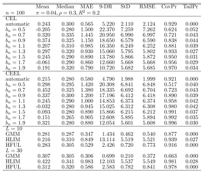
Mean Median MAE 9-DR StD RMSE CovPr TailPr
n= 100 = 0:04; = 0:3; R2 = 0:2 CEL
automatic 0.243 0.300 0.565 5.220 2.110 2.124 0.929 0.000
bn= 0:5 -0.205 0.280 1.500 22.370 7.259 7.262 0.624 0.052
bn= 0:7 0.320 0.335 1.445 20.950 6.990 6.997 0.721 0.043
bn= 0:9 0.374 0.325 1.150 18.650 6.579 6.590 0.838 0.044
bn= 1:1 0.207 0.310 0.985 16.350 6.249 6.252 0.881 0.039
bn= 1:3 0.297 0.320 0.930 15.060 5.795 5.802 0.933 0.027
bn= 1:5 0.245 0.290 0.890 13.780 5.866 5.872 0.950 0.031
bn= 1:7 -0.061 0.290 0.860 12.660 5.668 5.668 0.956 0.029
bn= 1:9 0.191 0.320 0.790 10.720 5.682 5.685 0.970 0.034 CEEL
automatic 0.215 0.280 0.580 4.790 1.988 1.999 0.921 0.000
bn= 0:5 0.298 0.295 1.420 20.308 6.841 6.848 0.517 0.040
bn= 0:7 0.452 0.325 1.380 18.335 6.692 6.704 0.723 0.043
bn= 0:9 0.337 0.300 1.200 17.196 6.412 6.418 0.890 0.039
bn= 1:1 0.245 0.290 1.000 14.853 6.373 6.374 0.958 0.042
bn= 1:3 -0.032 0.280 0.945 15.025 6.312 6.308 0.980 0.042
bn= 1:5 0.093 0.280 0.890 15.866 6.215 6.212 0.991 0.037
bn= 1:7 0.151 0.265 0.905 12.608 5.895 5.894 0.992 0.035
bn= 1:9 0.321 0.280 0.880 12.054 5.601 5.608 0.996 0.030
L= 10
GMM 0.281 0.287 0.347 1.434 0.462 0.540 0.877 0.000 HLIM 0.216 0.310 0.849 13.114 5.519 5.521 0.939 0.027 HFUL 0.283 0.305 0.529 2.426 0.720 0.773 0.916 0.000
L= 30
[image:22.595.96.493.271.609.2]GMM 0.307 0.305 0.306 0.699 0.210 0.372 0.663 0.000 HLIM 0.422 0.341 0.983 12.103 5.537 5.549 0.981 0.028 HFUL 0.312 0.320 0.586 2.583 0.782 0.841 0.978 0.000
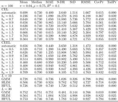
Mean Median MAE 9-DR StD RMSE CovPr TailPr
n= 100 = 0:04; = 0:75; R2 = 0:1 CEL
automatic 0.698 0.730 0.400 3.640 1.514 1.667 0.615 0.000
bn= 0:5 0.236 0.740 1.090 16.270 6.183 6.188 0.367 0.039
bn= 0:7 0.648 0.730 1.050 14.880 5.736 5.772 0.459 0.025
bn= 0:9 0.656 0.730 0.865 13.140 5.666 5.704 0.561 0.030
bn= 1:1 0.636 0.740 0.720 10.870 5.632 5.668 0.687 0.036
bn= 1:3 0.674 0.740 0.650 11.410 5.387 5.429 0.723 0.028
bn= 1:5 0.666 0.740 0.615 10.140 5.262 5.304 0.797 0.025
bn= 1:7 0.703 0.740 0.590 8.980 4.878 4.929 0.850 0.022
bn= 1:9 0.564 0.740 0.570 9.130 4.721 4.755 0.855 0.019 CEEL
automatic 0.656 0.700 0.440 3.650 1.318 1.472 0.656 0.000
bn= 0:5 0.528 0.710 1.200 14.490 5.683 5.705 0.357 0.029
bn= 0:7 0.626 0.740 1.235 13.808 5.965 5.994 0.481 0.037
bn= 0:9 0.736 0.700 1.050 12.498 5.762 5.806 0.577 0.033
bn= 1:1 0.514 0.695 0.980 10.802 5.490 5.511 0.651 0.031
bn= 1:3 0.460 0.680 0.950 10.330 5.489 5.506 0.712 0.034
bn= 1:5 0.408 0.680 0.940 9.837 4.861 4.861 0.761 0.023
bn= 1:7 0.558 0.695 0.930 8.847 4.393 4.426 0.807 0.016
bn= 1:9 0.709 0.700 0.930 8.105 4.713 4.763 0.832 0.022
L= 10
GMM 0.728 0.735 0.736 1.026 0.326 0.798 0.294 0.000 HLIM 0.506 0.730 0.924 9.782 4.702 4.727 0.718 0.020 HFUL 0.726 0.739 0.740 1.720 0.512 0.888 0.649 0.000
L= 30
[image:23.595.103.492.86.420.2]GMM 0.752 0.751 0.751 0.481 0.144 0.766 0.010 0.000 HLIM 0.564 0.751 1.004 8.534 4.908 4.938 0.822 0.025 HFUL 0.753 0.746 0.746 1.783 0.542 0.927 0.794 0.000
Mean Median MAE 9-DR StD RMSE CovPr TailPr
n= 100 = 0:4; = 0:3; R2= 0:2 CEL
automatic 0.001 0.040 0.235 1.360 0.461 0.461 0.953 0.000
bn= 0:5 -0.445 -0.010 0.405 5.160 3.587 3.614 0.711 0.014
bn= 0:7 -0.295 0.010 0.340 3.880 3.222 3.236 0.772 0.013
bn= 0:9 -0.147 0.010 0.260 1.910 1.577 1.583 0.868 0.003
bn= 1:1 -0.070 0.000 0.250 1.540 0.743 0.746 0.839 0.000
bn= 1:3 -0.059 0.000 0.240 1.510 0.588 0.591 0.895 0.000
bn= 1:5 -0.064 0.000 0.250 1.560 0.655 0.658 0.880 0.000
bn= 1:7 -0.070 0.000 0.255 1.570 0.794 0.797 0.913 0.000
bn= 1:9 -0.147 0.000 0.270 1.780 1.482 1.489 0.954 0.002 CEEL
automatic 0.018 0.030 0.240 1.340 0.451 0.451 0.956 0.000
bn= 0:5 -0.035 -0.020 0.330 3.093 2.688 2.686 0.665 0.008
bn= 0:7 -0.069 -0.010 0.300 2.422 2.176 2.176 0.757 0.005
bn= 0:9 -0.030 -0.020 0.250 1.671 1.201 1.201 0.872 0.000
bn= 1:1 -0.093 -0.010 0.230 1.541 1.646 1.647 0.922 0.004
bn= 1:3 -0.052 -0.015 0.240 1.511 0.573 0.575 0.947 0.000
bn= 1:5 -0.045 -0.010 0.245 1.511 0.581 0.582 0.958 0.000
bn= 1:7 -0.049 -0.010 0.250 1.563 0.690 0.692 0.975 0.000
bn= 1:9 -0.044 -0.010 0.265 1.630 1.303 1.304 0.985 0.001
L= 10
GMM 0.105 0.120 0.204 0.977 0.293 0.311 0.905 0.000 HLIM -0.012 0.023 0.315 2.396 2.242 2.241 0.938 0.005 HFUL 0.039 0.052 0.274 1.631 0.494 0.495 0.932 0.000
L= 30
[image:24.595.109.489.83.420.2]GMM 0.218 0.223 0.232 0.607 0.186 0.286 0.743 0.000 HLIM 0.014 0.061 0.479 5.169 3.685 3.684 0.976 0.013 HFUL 0.109 0.094 0.368 2.023 0.591 0.601 0.966 0.000
Mean Median MAE 9-DR StD RMSE CovPr TailPr
n= 100 = 0:4; = 0:75; R2 = 0:1 CEL
automatic 0.018 0.080 0.210 1.300 0.472 0.472 0.877 0.000
bn= 0:5 -0.605 -0.020 0.350 4.040 4.026 4.071 0.732 0.020
bn= 0:7 -0.485 -0.010 0.320 3.200 3.484 3.518 0.798 0.015
bn= 0:9 -0.218 -0.010 0.240 1.680 1.978 1.990 0.852 0.003
bn= 1:1 -0.172 -0.010 0.240 1.460 1.267 1.279 0.853 0.002
bn= 1:3 -0.143 -0.010 0.240 1.440 1.491 1.498 0.916 0.003
bn= 1:5 -0.140 -0.010 0.230 1.440 1.497 1.503 0.905 0.003
bn= 1:7 -0.088 -0.010 0.240 1.470 1.857 1.859 0.948 0.005
bn= 1:9 -0.037 0.000 0.250 1.530 1.502 1.503 0.959 0.002 CEEL
automatic 0.025 0.060 0.220 1.170 0.450 0.451 0.891 0.000
bn= 0:5 -0.333 -0.040 0.280 2.553 2.347 2.369 0.708 0.004
bn= 0:7 -0.209 -0.040 0.270 2.112 2.039 2.049 0.785 0.004
bn= 0:9 -0.109 -0.010 0.235 1.560 1.018 1.023 0.871 0.000
bn= 1:1 -0.073 -0.010 0.230 1.391 0.793 0.796 0.906 0.000
bn= 1:3 -0.085 -0.010 0.230 1.381 0.585 0.591 0.917 0.000
bn= 1:5 -0.055 -0.010 0.230 1.321 0.965 0.966 0.935 0.001
bn= 1:7 -0.080 -0.020 0.240 1.361 0.682 0.686 0.936 0.000
bn= 1:9 -0.035 -0.010 0.250 1.431 1.239 1.239 0.943 0.001
L= 10
GMM 0.295 0.311 0.320 0.779 0.244 0.383 0.633 0.000 HLIM -0.108 0.026 0.273 1.910 1.910 1.482 0.912 0.001 HFUL 0.067 0.093 0.230 1.136 0.372 0.378 0.892 0.000
L= 30
[image:25.595.105.491.84.423.2]GMM 0.532 0.533 0.533 0.470 0.144 0.551 0.073 0.000 HLIM -0.109 0.068 0.387 4.222 3.436 3.436 0.921 0.011 HFUL 0.202 0.181 0.267 1.449 0.441 0.485 0.907 0.000
A.2
n
= 200
Mean Median MAE 9-DR StD RMSE CovPr TailPr
n= 200 = 0:04; = 0:3; R2 = 0:2 CEL
automatic 0.287 0.275 0.505 4.080 1.588 1.614 0.869 0.000
bn= 0:3 -0.624 0.185 1.685 34.590 8.179 8.203 0.403 0.068
bn= 0:5 0.307 0.260 1.230 17.490 6.605 6.612 0.624 0.042
bn= 0:7 0.441 0.300 1.030 14.920 5.878 5.894 0.764 0.033
bn= 0:9 0.517 0.300 0.970 14.490 5.941 5.963 0.840 0.033
bn= 1:1 0.407 0.320 0.910 12.800 5.914 5.928 0.902 0.032
bn= 1:3 0.118 0.300 0.900 11.940 5.393 5.395 0.902 0.028
bn= 1:5 0.493 0.310 0.875 10.540 4.978 5.002 0.944 0.022
bn= 1:7 0.457 0.310 0.870 11.230 5.053 5.073 0.957 0.026 CEEL
automatic 0.362 0.300 0.540 4.710 1.820 1.855 0.851 0.000
bn= 0:3 0.353 0.325 1.400 18.294 6.511 6.517 0.283 0.034
bn= 0:5 0.381 0.290 1.160 17.738 6.509 6.517 0.663 0.037
bn= 0:7 0.297 0.250 1.085 16.777 6.322 6.326 0.850 0.036
bn= 0:9 -0.050 0.290 1.040 12.965 5.460 5.457 0.941 0.024
bn= 1:1 -0.009 0.300 1.035 13.601 5.489 5.487 0.961 0.026
bn= 1:3 0.153 0.290 1.020 13.518 5.584 5.583 0.980 0.027
bn= 1:5 0.245 0.295 1.020 12.366 5.751 5.753 0.986 0.032
bn= 1:7 0.092 0.275 0.960 12.436 5.615 5.613 0.991 0.032
L= 10
GMM 0.276 0.271 0.349 1.460 0.479 0.553 0.903 0.000 HLIM 0.542 0.285 0.836 13.919 5.466 5.490 0.944 0.025 HFUL 0.299 0.281 0.553 2.955 0.864 0.914 0.925 0.000
L= 30
[image:26.595.102.493.120.453.2]GMM 0.306 0.306 0.311 0.756 0.233 0.384 0.726 0.000 HLIM 0.411 0.383 0.988 12.625 5.331 5.344 0.966 0.025 HFUL 0.352 0.371 0.664 2.992 0.907 0.972 0.957 0.000
Mean Median MAE 9-DR StD RMSE CovPr TailPr
n= 200 = 0:04; = 0:75; R2 = 0:1 CEL
automatic 0.739 0.700 0.370 2.920 1.208 1.416 0.545 0.000
bn= 0:3 0.072 0.620 1.230 21.310 6.979 6.979 0.302 0.050
bn= 0:5 0.640 0.690 0.870 14.260 6.059 6.093 0.434 0.042
bn= 0:7 0.650 0.695 0.745 10.990 5.230 5.271 0.510 0.026
bn= 0:9 0.642 0.680 0.705 11.560 5.290 5.329 0.637 0.026
bn= 1:1 0.633 0.690 0.675 10.070 5.243 5.282 0.725 0.026
bn= 1:3 0.589 0.675 0.635 8.800 4.724 4.760 0.731 0.020
bn= 1:5 0.641 0.680 0.620 8.560 4.571 4.615 0.791 0.022
bn= 1:7 0.685 0.680 0.610 7.910 4.403 4.456 0.801 0.019 CEEL
automatic 0.717 0.720 0.420 3.720 1.331 1.512 0.584 0.000
bn= 0:3 0.726 0.730 1.240 14.034 5.555 5.600 0.256 0.023
bn= 0:5 0.781 0.690 1.075 13.467 5.622 5.674 0.425 0.028
bn= 0:7 0.377 0.645 1.060 12.371 5.343 5.353 0.542 0.023
bn= 0:9 0.361 0.660 1.050 10.564 4.659 4.671 0.621 0.017
bn= 1:1 0.507 0.685 1.030 11.054 4.769 4.794 0.681 0.019
bn= 1:3 0.599 0.690 1.020 10.838 5.109 5.142 0.736 0.024
bn= 1:5 0.547 0.680 1.020 10.252 4.769 4.797 0.782 0.020
bn= 1:7 0.512 0.685 1.010 8.905 4.608 4.634 0.819 0.019
L= 10
GMM 0.720 0.722 0.722 1.033 0.339 0.796 0.345 0.000 HLIM 0.758 0.707 0.892 9.010 4.581 4.651 0.694 0.017 HFUL 0.731 0.715 0.722 2.115 0.621 0.959 0.649 0.000
L= 30
[image:27.595.104.492.86.420.2]GMM 0.749 0.752 0.752 0.537 0.163 0.767 0.021 0.000 HLIM 0.613 0.770 1.025 9.232 4.492 4.531 0.779 0.015 HFUL 0.776 0.769 0.775 2.133 0.643 1.007 0.747 0.000
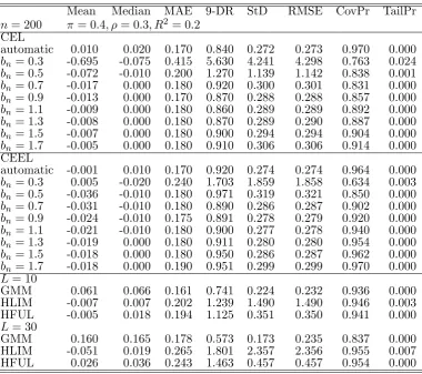
Mean Median MAE 9-DR StD RMSE CovPr TailPr
n= 200 = 0:4; = 0:3; R2= 0:2 CEL
automatic 0.010 0.020 0.170 0.840 0.272 0.273 0.970 0.000
bn= 0:3 -0.695 -0.075 0.415 5.630 4.241 4.298 0.763 0.024
bn= 0:5 -0.072 -0.010 0.200 1.270 1.139 1.142 0.838 0.001
bn= 0:7 -0.017 0.000 0.180 0.920 0.300 0.301 0.831 0.000
bn= 0:9 -0.013 0.000 0.170 0.870 0.288 0.288 0.857 0.000
bn= 1:1 -0.009 0.000 0.180 0.860 0.289 0.289 0.892 0.000
bn= 1:3 -0.008 0.000 0.180 0.870 0.289 0.290 0.887 0.000
bn= 1:5 -0.007 0.000 0.180 0.900 0.294 0.294 0.904 0.000
bn= 1:7 -0.005 0.000 0.180 0.910 0.306 0.306 0.914 0.000 CEEL
automatic -0.001 0.010 0.170 0.920 0.274 0.274 0.964 0.000
bn= 0:3 0.005 -0.020 0.240 1.703 1.859 1.858 0.634 0.003
bn= 0:5 -0.036 -0.010 0.180 0.971 0.319 0.321 0.850 0.000
bn= 0:7 -0.031 -0.010 0.180 0.890 0.286 0.287 0.902 0.000
bn= 0:9 -0.024 -0.010 0.175 0.891 0.278 0.279 0.920 0.000
bn= 1:1 -0.021 -0.010 0.180 0.900 0.277 0.278 0.940 0.000
bn= 1:3 -0.019 0.000 0.180 0.911 0.280 0.280 0.954 0.000
bn= 1:5 -0.018 0.000 0.180 0.950 0.286 0.287 0.962 0.000
bn= 1:7 -0.018 0.000 0.190 0.951 0.299 0.299 0.970 0.000
L= 10
GMM 0.061 0.066 0.161 0.741 0.224 0.232 0.936 0.000 HLIM -0.007 0.007 0.202 1.239 1.490 1.490 0.946 0.003 HFUL -0.005 0.018 0.194 1.125 0.351 0.350 0.941 0.000
L= 30
[image:28.595.109.490.83.420.2]GMM 0.160 0.165 0.178 0.573 0.173 0.235 0.837 0.000 HLIM -0.051 0.019 0.265 1.801 2.357 2.356 0.955 0.007 HFUL 0.026 0.036 0.243 1.463 0.457 0.457 0.954 0.000
Mean Median MAE 9-DR StD RMSE CovPr TailPr
n= 200 = 0:4; = 0:75; R2 = 0:1 CEL
automatic 0.041 0.050 0.160 0.840 0.284 0.287 0.893 0.000
bn= 0:3 -0.821 -0.040 0.345 5.150 4.724 4.794 0.769 0.031
bn= 0:5 -0.067 -0.010 0.190 1.170 1.060 1.062 0.853 0.001
bn= 0:7 -0.045 -0.010 0.160 0.820 0.270 0.274 0.853 0.000
bn= 0:9 -0.039 -0.010 0.160 0.790 0.263 0.266 0.885 0.000
bn= 1:1 -0.036 -0.010 0.160 0.780 0.259 0.262 0.904 0.000
bn= 1:3 -0.033 -0.010 0.160 0.770 0.259 0.261 0.906 0.000
bn= 1:5 -0.031 -0.010 0.160 0.770 0.261 0.263 0.911 0.000
bn= 1:7 -0.030 0.000 0.160 0.790 0.265 0.267 0.966 0.000 CEEL
automatic 0.006 0.020 0.150 0.810 0.252 0.252 0.930 0.000
bn= 0:3 -0.061 -0.020 0.195 1.431 1.846 1.846 0.687 0.004
bn= 0:5 -0.067 -0.020 0.160 0.880 0.342 0.349 0.886 0.000
bn= 0:7 -0.050 -0.010 0.150 0.820 0.265 0.270 0.919 0.000
bn= 0:9 -0.044 -0.010 0.150 0.810 0.248 0.252 0.938 0.000
bn= 1:1 -0.041 -0.010 0.150 0.791 0.248 0.251 0.942 0.000
bn= 1:3 -0.040 -0.010 0.150 0.810 0.250 0.253 0.946 0.000
bn= 1:5 -0.039 -0.010 0.150 0.810 0.254 0.257 0.958 0.000
bn= 1:7 -0.039 -0.010 0.160 0.821 0.260 0.263 0.964 0.000
L= 10
GMM 0.168 0.184 0.203 0.622 0.191 0.254 0.780 0.000 HLIM -0.050 0.011 0.183 0.975 0.341 0.344 0.934 0.000 HFUL -0.002 0.039 0.178 0.854 0.273 0.273 0.925 0.000
L= 30
[image:29.595.104.490.86.418.2]GMM 0.390 0.394 0.394 0.439 0.132 0.412 0.200 0.000 HLIM -0.080 -0.016 0.217 1.359 1.043 1.046 0.946 0.001 HFUL -0.008 0.028 0.203 1.005 0.337 0.337 0.936 0.000
Table 8: strong instruments, high endogeneity
B
Appendix: Notes on computation
B.1
Lagrange multipliers for CEL
The Lagrange multiplier (zi; )is the solution, for anyi= 1; :::; n, of the maximization problem
(zi; ) = arg max
n
X
j=1
wijlog (1 + g(yj; xj; )):
For simplicity of notation drop the subscript ifromwij and let gj =g(yj; xj; ). Then, the Lagrange multiplier corresponding to this generic case is found by maximizing
f( ) =
n
X
j=1
wjlog (1 +gj ):
This is a function strictly concave in unless gj = 0 for all j.
maxng1
jjgj >0; wj >0 o
<0andd= minng1
jjgj <0; wj >0 o
>0;6 then forc < < d
it holds that 1 +gj > 0 for all j. We use the Newton-Raphson algorithm to …nd the Lagrange multiplier. In order to ensure that the algorithm does not take values outside the interval(c; d), we maximize in fact the function
F (t) =
n
X
j=1
wjlog 1 +gj
c+det
1 +et ; t2R;
suppose we obtaint = arg maxtF (t). Then, the Lagrange multiplier is determined as
= c+de
t
1 +et 2(c; d):
This method for computing the Lagrange multipliers (zi; ) has worked very well for our DGP’s.
B.2
Cross-validation
The cross-validation criterion proposed by Newey (1993, p.433) adapted to our model is
d
CV (bn) = n
X
i=1
b
R2(zi) (zi);
where
b
R(zi) =
n b
D(zi) D(zi) +B(zi)
h
b(zi) (zi)
io
;
B(z) = D(z) (z) 1 and Db(z), b(z) are nonparametric kernel regression estimators of D(z), (z), respectively, where
D(z) = E @g(y; x; 0)
@ jz ; (z) =E g
2(y; x;
0)jz :7 (7) The expressionRb(zi) cannot be computed; Newey proposes to estimate it by
R(zi) =
2
4@g yi; xi;b
@ Db i+Bb i bg
2 i b i
3 5;
6Note that, since we use the Epanechnikov kernel, not all weightsw
jare necessarily strictly positive.
7For our DGP these expressions are
D(z) = E[ xjz] = z;
(z) = E 2
4 u+
s
1 2
2+:864( v1+:86v2)
!2 jz
3
where Db i and b i are leave-one-out estimators of D(zi)and (zi). Speci…cally,
b
D i =
n
X
j=1; j6=i
xjw ij;
b i = n
X
j=1; j6=i
b
g2jw ij;
b
B i = Db ib 1i;
where
w ij =
K zi zj
bn Pn
j=1; j6=iK zi zj
bn
;
b
gi = g yi; xi;b :
The basic idea underlying this estimation is to replace the conditional expectations by their leave-one-out estimators and the estimators of the conditional expectations by the dependent variables in the associated nonparametric regression. In our model the criterion simpli…es to
R(zi) =
" b
D i b
g2 i
b i 1 !
xi Db i
#
:
The cross-validation criterion we use is
CV (bn) = n
X
i=1
R2(zi)b i:
References
[1] Antoine, B., H. Bonnal, E. Renault (2007): On the E¢cient Use of the Infor-mational Content of Estimating Equations: Implied Probabilities and Euclidean Empirical Likelihood, Journal of Econometrics, 138, 461-487.
[2] Domínguez, M. A., I. N. Lobato (2004): Consistent Estimation of Models De…ned by Conditional Moment Restrictions, Econometrica, 72, 1601-1615.
[3] Fiebig, D. G. (1985): Evaluating Estimators without Moments, The Review of Economics and Statistics,67, 529-534.
[4] Fuller, W. A. (1977): Some Properties of a Modi…cation of the Limited Information Estimator, Econometrica, 45, 939-953.
[5] Gospodinov, N. and T. Otsu (2009): Local GMM Estimation of Time Series Models with Conditional Moment Restrictions, forthcoming Journal of Econometrics.
[6] Guggenberger, P. (2008): Finite Sample Evidence Suggesting a Heavy Tail Problem of the Generalized Empirical Likelihood Estimator, Econometric Reviews,27, 526-541.
[7] Hansen, L. P. J. Heaton, A. Yaron (1996): Finite-Sample Properties of Some Alter-native GMM Estimators,Journal of Business and Economic Statistics,14, 262-280.
[8] Hausman, J. A., W. K. Newey, T. Woutersen, J. Chao, N. Swanson (2010): In-strumental Variable Estimation with Heteroskedasticity and Many Instruments, mimeo.
[9] Kitamura, Y., G. Tripathi, H. Ahn (2004): Empirical Likelihood-Based Inference in Conditional Moment Restriction Models, Econometrica,72, 1667-1714.
[11] Newey, W. K. (1993): E¢cient Estimation of Models with Conditional Moment Restrictions, in Handbook of Statistics, 11, ed. by G. Maddala, C. Rao, and H. Vinod, Elsevier, 2111-2245.
[12] Smith, R. J. (2007): E¢cient Information Theoretic Inference for Conditional Mo-ment Restrictions,Journal of Econometrics, 138, 430-460.
[13] Tripathi, G., Y. Kitamura (2003): Testing Conditional Moment Restrictions, The Annals of Statistics, 31, 2059-2095.