The Baby Boom, Baby Busts, and Grandmothers

Munich Personal RePEc Archive

The Baby Boom, Baby Busts, and

Grandmothers

Orman, Cuneyt and Goksel, Turkmen and Gurdal, Mehmet

Y

Central Bank of the Republic of Turkey, Ankara University, TOBB

University of Economics and Technology

January 2011

The Baby Boom, Baby Busts, and Grandmothers1

Turkmen Goksel2, Mehmet Y. Gurdal3, and Cuneyt Orman4

First version: December 2009

This version: January 2011

Abstract

Studies in family economics and anthropology suggest that grandmothers are a highly valuable

source of childcare assistance. As such, availability of grandmothers affects the cost of having

children, and hence fertility decisions of young parents. In this paper, we develop a simple

model to assess the fertility implications of the fluctuations in both output (as argued by

demographers) and grandmother-availability induced child-care costs over the period

1920-1970. Model does a good job of mimicking the bust-boom-bust pattern during this period. When

the child-care cost channel is shut down, the model’s performance weakens significantly; in

particular, it fails to capture the bust in the 1960’s altogether.

JEL Classification Numbers: J13, J20

Keywords: fertility, baby boom, baby bust, female labor-force participation, grandmother

availability

1

We thank seminar participants at Turkish Economic Association’s International Conference on Economics in Girne and Middle East Economic Association’s Meeting in Istanbul, and two anonymous referees for helpful comments and suggestions. All remaining errors are our own. The views expressed herein are solely of the authors and do not represent those of the Central Bank of the Republic of Turkey or its staff.

2

Department of Economics, Ankara University, Cemal Gursel Bulvari, 06590 Cebeci, Ankara, TURKEY 3

Department of Economics, TOBB University of Economics and Technology, Sogutozu Cad. 43, 06560 Sogutozu, Ankara, TURKEY

4

1. Introduction

During the 20th century, fertility in the United States, and in many other industrialized nations,

has exhibited a series of unprecedented deviations around an otherwise declining trend. The

most striking of these deviations is the large upward swing in fertility beginning roughly in the

early 1940's and lasting until the early 1960's. This “baby boom” was followed by a sharp

downturn after the early 1960's, the “baby bust”, which brought fertility back to trend by the

1980's.

Existing theories of the baby boom and baby bust often attribute these events to fluctuations in

productivity that occurred with similar timing - the boom following World War II and the

slowdown of the 1970's. Quantitative models appear to lend some support to these theories, but

they also suggest that productivity fluctuations are only part the story. Calibrating a model that

combines simple versions of the stochastic growth model and the Barro-Becker model of

endogenous fertility, Jones and Schoonbroodt (2007) find that deviations in productivity capture

about 40 percent of the baby boom. Their model, however, predicts the continuation of the boom

well into the 1960’s, which is in stark contrast with the data. Greenwood et al. (2005) take into

account the fertility implications of deviations in household sector productivity in addition to

those in market sector productivity. They argue that the introduction of electricity and associated

household appliances reduced the need for labor in the child-rearing process; the implied lower

cost of having children must then have led to an increase in fertility, and hence the baby boom.

This idea is subsequently quantified in a model that combines elements of the standard

overlapping-generations model of population growth and a standard household production

model. Although the pattern of fertility generated by their preferred model matches the long-run

trend in the U.S. data, the model underestimates the baby boom. An alternative specification of

their model provides a better match to the boom, but it also causes the model to underestimate

the decline in fertility during the baby bust.

Doepke et al. (2005) propose an alternative theory based on increased demand for female labor

during World War II. They argue that women who were old enough to work during the war

after the war. Younger women who turned adult only after the war and entered the labor market

faced competition not only from the men who returned from the war but also from the

experienced women of the war generation who were still in the labor force. They argue that this

led to less demand for inexperienced young women, who were crowded out of the labor market

and chose to have more children instead; and that it is these younger women who account for the

bulk of the baby boom. They formalize these ideas in a model of fertility choice along the lines

of Galor and Weil (1996) and find that the mechanism can account for a substantial portion of

the baby boom and bust event.

A main weakness in most of the papers in this literature is their inability to capture the baby bust

occurring in the 1960s: While some models underestimate the baby bust, others fail to capture it

altogether, driving fertility the wrong way. In this paper, we argue that incorporating the changes

in the availability of extended family members such as aunts and grandmothers and female

neighbors and friends for child-rearing that took place during this period into these models can

improve their match with the data, particularly in the bust period. The basic idea is that the

availability of aunts, grandmothers, and friends (henceforth “grandmother availability” for short)

in the home or vicinity should reduce the cost of having kids and hence cause an increase in

fertility, other things constant. Since there was a sharp drop in grandmother availability between

the late 1950s and the late 1960s after half a century of roughly constant levels (as will be

argued in sections 2 and 4), the cost of having kids must have gone up sharply in this period,

potentially leading to a bust in fertility.

In order to find out if this hypothesis has any promise confronting the data, at least in a

qualitative sense, we use a simple model of fertility along the lines of Yasuoka and Miyake

(2009) in which fertility is determined jointly by fluctuations in productivity and child-care

costs. The novel aspect of our approach is that we assume that fluctuations in child-care costs are

generated by fluctuations in grandmother availability. In particular, following Heckman (1974)

and others in the family economics literature, we postulate a negative relationship between the

two variables, whereby higher (lower) levels of grandmother availability are associated with

lower (higher) levels of child-care costs. After quantifying the model using U.S. data, we find

period 1920-1970, thereby replicating the well-known bust-boom-bust pattern, but that there are

differences in the levels of the two series.5 When we shut down the child-care cost channel

induced by movements in grandmother availability, the match between the model-generated and

actual fertility series worsens considerably and the model fails to capture the baby bust in the

1960’s altogether, driving fertility the wrong way. We interpret these findings as evidence that

fluctuations in child-care costs induced by movements in availability of grandmothers play a

particularly important role in the baby bust event of the 1960’s.

The remainder of the paper is organized as follows. In the next section, we first provide

empirical evidence concerning trends in grandmother availability for child-care assistance. We

also shed some light on the reasons causing the drastic change in the availability of

grandmothers that took place during the 10-15 year period following the late 1950’s. We then

present both theoretical and empirical evidence on the relationship between grandmother

availability, child-care costs, female labor force participation, and fertility. In Section 3, we

develop the formal model of the relationship between fertility, productivity, child-care costs, and

grandmother availability. A series of quantitative experiments are conducted on our theoretical

model in Section 4. This section also introduces our formal definition of grandmother

availability and explains how we measure it from data. Section 5 presents concluding remarks.

2. Theoretical and Empirical Evidence

2.1. Changes in Grandmother Availability

We hypothesize that (i) grandmothers will be less likely to offer help in child-rearing if they are

working or looking for work themselves, and (ii) mothers will be more likely to need child-care

assistance if they are working or looking for work themselves. In order to get a quantitative

measure of grandmother availability for child-care assistance over time, we utilize Census data

from the Integrated Public Use Microdata Series (IPUMS) of the Minnesota Population Center.

This data set provides information on labor force participation rates of women for various age

5

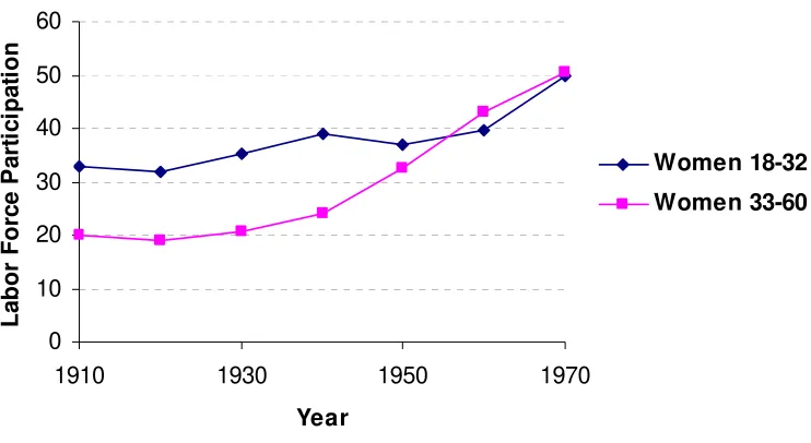
groups on a decennial basis. Figure 1 displays the evolution of the labor force participation rates

of young-age (18-32 years) and old-age (33-60 years) females between 1910 and 1970.

0 10 20 30 40 50 60

1910 1930 1950 1970

Year L a b o r F o rc e P a rt ic ip a ti o n Women 18-32 Women 33-60

Figure 1: Labor Force Participation by Young (18-32) and Old (33-60) Women in the United States (includes women of all races and marital statuses)

The figure indicates that between 1910-1970 (i) labor force participation rates for both young

and old-age females increased almost steadily, with roughly equal growth rates until the 1940's

and (ii) the labor force participation rate of older women (33-60) grew more rapidly than that of

younger women (18-32) beginning in the 1940's. Therefore, the symmetric evolution of the labor

force participation of younger and older women goes through a breakdown around 1940.6 If we

assume that the young-age women represent potential mothers and the old-age women represent

potential grandmothers in the population, these two observations suggest a simultaneous

increase in the need for non-parental child-care (potential moms are more likely to be working)

and a decrease in the availability of such care (potential grandmothers are more likely to be

working) over time. Therefore, non-parental child-care provided by grandmothers becomes

increasingly scarce during this period. Moreover, the increase in the scarcity of such care

accelerates in the 1950's. In the absence of other forms of child-care, such as those provided in

6

formal markets, the decline in grandmother availability must have worked to increase the cost of

having kids between 1910 and 1970, particularly after the early 1950's.

2.2. Formal Child-care Availability before the 1970's

In our analysis, we focus on the period before 1970. The scarce evidence suggests that the size

of the (formal) child-care industry was quite small up until the early 1970's. For example, Low

and Spindler (1968) find in their survey that in 1965, for 10.5 million mothers with children 0-17

years of age, licensed day care facilities were available for only 475,000 children. They also

report that 80 percent of children were cared for either by themselves, or by their immediate or

extended family (mother, father, or other relative). Ruderman (1968) reports similar findings

concerning the forms of child-care available during that period. Kamerman (1983), on the other

hand, provides evidence to the effect that the child-care industry grew rapidly beginning in the

early-to-mid 1970s. An important factor contributing to this change appears to have been the

government programs (such as workfare legislations and child-care tax credits) initiated in the

early 1970's under the Nixon administration. Since these programs subsidize market-provided

child care, but not that provided by unpaid relatives, they change the relative price of market and

nonmarket provided care (Klerman and Leibowitz, 1990). This change coupled with the fact that

labor force participation by women has also been growing seems to have been an important

force behind the rapid growth of the child care industry observed in the 1970's.

2.3. Child-care Availability, Grandmothers, and Employment Decisions

Previous research shows that child care costs have a significant effect on the employment

decisions of women. Low and Spindler (1968) report that the younger the children the less likely

was a mother to be working a full year rather than part year. Ruderman (1968), Bowen and

Finegan (1969), and Gronau (1973) find that only younger children (under 3) exert an important

retarding effect on women's work effort. These findings might be explained by the fact that

child-care costs are the highest for this group of children (See, for example, Del Boca et. al.,

Child care costs also affect the fertility decisions of women. Blau and Robins (1989, 1990)

provide evidence that fertility is negatively related to the price of child care. Connelly (1992)

finds that fertility and employment decisions are intertwined and that higher child care costs

discourage employment.

In the absence of a formal child care market, other arrangements for child care become important

in determining the fertility and employment decisions of young women. Low and Spindler

(1968) report that 80 percent of children of working mothers were cared for by themselves or by

their immediate or extended family and that the most frequent type of child care used was by a

relative other than the father, and that a substantial fraction of that care was provided by

grandparents (presumably grandmothers). They also report that the lowest level of

dissatisfaction for care provided by people other than themselves was about care provided by

other adult relatives such as the grandmothers. Rodes (1975) reports a similar finding concerning

care provided by adult relatives. Consistent with this body of work, Mason and Kuhlthau (1992)

find in their sample of working mothers that about one-third name relatives such as the

grandmother rather than the child's father as the ideal caregiver for children under age three.

There is also evidence that the presence of the grandmother in the household is associated with

higher likelihoods of being in the labor market (Van Gameren and Ooms, 2009), and earlier

returns to work among working women with preschool-aged children, especially those with

young preschoolers (Klerman and Leibowitz, 1990). Among those returning to work before their

infant was three months old, more than half the women used a relative to care for their child

(Leibowitz et al., 1992). They also report that having one's own mother nearby has a large

impact on the types of child care chosen for very young. However, later decisions about type of

provider are independent of the availability of the grandmother.

2.4. Arguments from Anthropology

The evidence coming from studies in anthropology confirms the effect of grandmothers on

fertility decisions of young women. These studies are mainly motivated by the observation that a

major difference between human beings and other mammals is that female members of human

reproductive and postmenopausal life spans of human species with other primates. Although

different primates have reproductive phases of same lengths during their life time, female human

species have exceptionally long postmenopausal life spans (Schultz, 1969).

A proposed explanation for this phenomenon, Grandmothering Hypothesis, suggests that

post-reproductive component of life for females is favored by natural selection due to positive effects

of grandmothering on the fitness of the offspring (Hawkes et al., 1998). This effect has likely

emerged as human societies were shifting from simple to hard-to-handle food, giving an

opportunity to vigorous elder females for helping their daughters and increasing the

representation of their vigor in descendant generations (Hawkes, 2004).

Using individual-based multi-generational data sets from pre-modern (18th and 19th centuries)

populations of Finland and Canada, Lahdenpera et al. (2004) study the fitness benefits of

post-reproductive lifespan for females. They find that the presence of a grandmother increases the

number of grandchildren and reduces interbirth intervals for the grandchildren. In addition to

this, grandchildren have significantly higher survival probabilities if their grandmother is alive at

their birth.

3. The Model

In this section, we lay out a model of the response of fertility to movements in Total Factor

Productivity (TFP) and grandmother availability. The model we use is based on Yasuoka and

Miyake (2009). We add two new components to the basic model: Productivity shocks and

child-care cost shocks, where the latter is assumed to be induced by changes in grandmother

availability. In each period, the shocks are realized and the representative household decides

how much to consume, how many children to have, and how much to invest in each child's

education given her income.7 Income is determined by the household's human capital level and

the realization of the productivity shock. The household's human capital, in turn, depends on her

7

parents' human capital and on her level of education (chosen by her parents in the previous

period)

The household's problem can be formulated as follows. In each period, the household solves the

utility maximization problem:

) ln( ) 1 ( ) ln(

max ₁

,

,n e t t t

c_{t t t}α nh+ + −α c

subject to:

t t t t t t

tn e n c s h

p + + = (1)

h_t+1 =e_tβh_t1−β (2)

h₀ fixed,

where st is the productivity shock, pt is the child-care cost, ct is consumption, nt is the

number of children, e_t is the level of education per child, h_t is human capital in period t and

α andβare between 0 and 1. The maximization takes place after the realization of s_t andp_t.

Equation (1) is the budget constraint and equation (2) is the law of motion for human capital

across generations.8

There are two types of costs associated with having children and, for simplicity, both costs are

assumed to be in terms of goods. The first cost, p_t is associated with producing children and is

best interpreted as representing child-related costs that begin around birth and continue during

the early preschool years of a child. The key assumption we make is that if a grandmother is

around to help with looking after children, then this cost is reduced for parents. We model this

effect by letting pt be a decreasing function of grandmother availability, Gt that is, we let

8

pt = f(Gt), (3)

where f(.)>0 and f'(.)<0.9The second cost of having children is associated with educating

them. In particular, parents can increase the quality of a given child (i.e. the human capital in the

following period) by spending resources: At a cost of e_t the human capital of a child can be

increased from h_tto h_t+1 according to equation (2). We assume that this cost is independent of

grandmother availability.

The solution for the optimization problem stated above yields the following optimal allocations:

c_t =(1−α)s_th_t, (4)

β β

− =

1 t t

p

e , (5)

t t t t

p h s

n =α(1−β) . (6)

The key variable of interest is the fertility rate, nt, given by equation (6). This is the model

quantity that we will identify with the Total Fertility Rate (TFR) in the data in the next section.

Note that n_t increases with the realized level of income, s_th_t, and decreases with the cost of

producing children, p_t.10 Moreover, the law of motion for human capital implies that h_t

depends on the initial level of human capital and the past realizations of the cost of producing

children in the following way:

9

In Yasuoka and Miyake (2009)'s theoretical model, the price of child-care is determined endogenously by supply and demand in a formal market for child-care services.

10

Assuming that fertility is increasing in income might seem strange in the face of the fact that most studies find a negative relationship between the two variables; especially if one is trying to understand the secular decline in fertility rates in industrialized countries since the early 1800’s. Since our focus is on the period between 1910 and 1970, however, we do not view this as a serious problem for our analysis. This is because the coefficient of correlation between the two annual series for TFR and TFP for the years 1917 to 1968 is 0.35, which suggests that the U.S. TFR is procylical during this period. Please see also Jones and Schoonbroodt (2007) on this point, who find that the coefficient of correlation between the annual series of the deviations of the two variables from their

o t t t t t t h p p p h

h (1 )

1 ) 1 ( 0 0 ) 1 ( 1 1 1 1 ... 1 ) ( β β β β β β β β β − − − − − − − ⎟⎟ ⎠ ⎞ ⎜⎜ ⎝ ⎛ − ⎟⎟ ⎠ ⎞ ⎜⎜ ⎝ ⎛ − =

= , (7)

where pt−1 =(p_t−1,p_t−2,...,p_o) is the history of child-care costs up to and including period t−1.

Taking account of this, equation (6) can be rewritten as

t t t t t p p h s

n (1 ) ( )

1 −

−

=α β . (8)

Therefore, both current and past realizations of p influence nt, but they do so in a different

way. Specifically, while high values of current preduce n_t, high values of past p's increase it.

It is easy to see why a high p_t should reduce n_t: The high cost of having kids discourages

parents from having too many. To see why high values of past p's increase n_t on the other

hand, consider the following thought exercise: Suppose that p_t−1 is high. In this case, the high

cost of producing kids discourages parents from having kids in period t−1, causing n_t−1 to go

down (equation 6). The reduction in the number of kids then relaxes period t−1 parents' budget

constraint and allows them to spend more on each child's education, increasing et₋₁ (equation 5).

Increased child education in period t−1 produces higher human capital adults (i.e. parents) in

period t, causing h_t to go up (equation 2). This, in turn, allows period t parents to earn more

income. Since children are normal goods, the increase in income leads to an increase in number

of children in this period, that is, a higher n_t (equation 6). This result can be interpreted as a

Beckerian quantity-quality trade-off.

4. Quantification

In this section, we perform a number of simple quantitative experiments on the model developed

in the previous section. Our ultimate goal is to find out whether including grandmother

availability in an otherwise standard model of fertility choice can improve the ability of the

we first calculate the actual magnitudes of deviations from the trends of TFP and child-rearing

costs for every decade from the 1910's to the 1960's, and then feed these into the model to obtain

model results for fertility rates. Next, we compare the fertility series generated by the model with

the actual time series of fertility rates. Finally, in order to highlight the significance of

child-rearing costs for fertility, we consider a version of the model in which shocks to child-child-rearing

costs are completely shut down, and compare the results with that of the full-fledged model.

While performing these exercises, we also briefly describe the main features of the relevant

variables in the data, namely, TFP, TFR, and availability of child-care assistance provided by

grandmothers.

4.1 Model with both TFP and Child-rearing Cost Shocks

A critical choice here is the length of a period. Like Greenwood et al. (2005) and Jones and

Schoonbroodt (2007), we assume that a period is 10 years. In addition, we must specify the

parameters of the model to fully characterize the decision rules. Throughout, we set α =1/2 and

2 / 1 =

β .11 Finally, we normalize the initial levels of human capital and child-rearing costs to 1,

that is, we set h₀ = p_o =1.

Next, we must obtain the realizations of the shocks to TFP and child-rearing costs for all decades

beginning with 1910-1919 and ending with 1960-1969. To this end, we first use the TFP data as

laid out in Kendrick (1961) and Kendrick (1973). This data series is available at annual

frequencies and is shown in Figure 2 over the period 1889 to 1969.

11

0 50 100 150 200 250

1889 1899 1909 1919 1929 1939 1949 1959 1969

Year

T

F

P

I

n

d

ex,

1929 =

100

Figure 2: Total Factor Productivity, 1889-1969

The main features of this data series are:

• A general upward trend,

• An downward trend during the 1920's and 1930's, and

• A return to trend following World War II.

We use this data series to obtain the realizations of the TFP shocks for the period 1910-1970. In

particular, we first define

t t t

A A

s = (9)

where A_tdenotes the realization of TFP in period t and A_t denotes the value predicted by the

trend of TFP in period t. Thus, s_t takes the value of 1 if there is no shock, that is, when

t

t A

A = . Depending on the nature of the shocks, which can be positive or negative, the value of

t

s moves around 1. Note that while A_t comes directly from Kendrick's data, A_t must be

to compute s_tdecade by decade, beginning with 1910 to 1919. The estimated series for s_t is

given by [0.935, 0.966, 0.905, 0.987, 1.026, 1.079].

Obtaining the series for the child-rearing costs, p_t, is slightly more involved. We do this in a

number of steps. First, recall that we argued in the previous sections that child-rearing costs are

negatively related to grandmother availability. Here, we specify this relation as

) ( )

(

_

t t

t f G p G

p = = +ε (10)

where

_

p is the constant long-run level of the child-care cost, which is without loss of insight set

equal to po (which is equal to 1 by assumption), and ε(Gt) is the shock to this cost induced by

movements in grandmother availability. Therefore, we assume that changes in the cost of

child-care come only from changes in the availability of grandmothers for child-rearing.12 Just like the

value of s_t, the value of p_t moves around 1: While an above-trend value of G_tdecreases p_t (in

which case ε(G_t)<0), a below-trend value of G_t increases it (in which case ε(G_t)>0).

In order to determine whether ε(G_t) is positive or negative, we must first obtain a quantitative

measure of grandmother availability, G_t. Unfortunately, grandmother availability is not a

routinely reported statistic. We must therefore construct it ourselves. Our approach to

constructing such a measure is based on two premises:

• Grandmothers will be more likely to offer child-care assistance if they are not working or

looking for work, and

• Mothers will be more likely to need child-care assistance if they are working or looking

for work.

12

Consistent with these premises, we use labor force participation data for younger and older

women (representing potential mothers and potential grandmothers, respectively) from IPUMS

for the decades 1910 to 1970 to construct our statistic.13 In particular, we compute

(

)

(

)

t t between aged are and force labor the in who Women between aged are and force labor the in who Women G 32 -18 60 -33 are not are =

for t=1910-1919,...,1960-1969. Here, the numerator is used as a proxy for the supply of child-care and the denominator as a proxy for the demand for child-care. As such, this statistic can be interpreted as an “effective supply” or “availability” of child-care assistance provided by

grandmothers in the present context.14 Note that by construction this measure takes into account

child-care assistance provided not only by extended family members such as aunts and

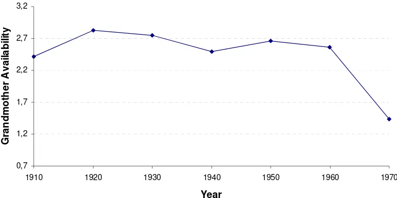
grandmothers, but potentially also that provided by female neighbors or friends. Figure 3 shows

the time path for this series. Observe that the availability of child-care assistance is essentially

constant between 1910 and 1960, with a sharp decline thereafter. As we will see shortly, this

change likely has important implications for trends in fertility.

13

Note that since IPUMS dataset is based on Census surveys, the data are available only every 10 years. Also, since this dataset comes from a stratified sample, the data are weighted using the appropriate weighting scheme. See Ruggles et al. (2004) for details.

14

0,7 1,2 1,7 2,2 2,7 3,2

1910 1920 1930 1940 1950 1960 1970

Year

G

ra

ndm

ot

he

r A

v

a

il

a

bi

li

ty

Figure 3: Grandmother Availability

Having developed the grandmother availability statistic, we are ready to define ε(G_t) which

was first introduced in equation (10). First, using the fact that Gt is roughly constant during

most the period between 1910 and 1970, we take the average of the values for 1910-1970 in

order to obtain the “trend” value of Gt for the period.

15

Let G denote this trend value.We can

then define

( )= −1 t t

G G G

ε (11)

Observe that ε(G_t)>0 when G_t <G and ε(G_t)<0 when G_t >G . We finally use equation

(11) in conjunction with equation (10) to compute p_t decade by decade, beginning with 1910 to

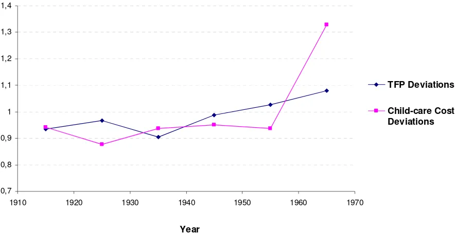
1919. The estimated series for p_t is given by p =[0.941, 0.878, 0.937, 0.952, 0.938, 1.329].

The following figure shows the deviations of s_t and p_t from their respective trends.

15

0,7 0,8 0,9 1 1,1 1,2 1,3 1,4

1910 1920 1930 1940 1950 1960 1970

Year

TFP Deviations

Child-care Cost Deviations

Figure 4: Total Factor Productivity and Child-care Cost: Deviations from Trend

The final step in our experiment is to compare the model-generated fertility series versus the

actual time series of fertility rates. To do this, we first obtain model results for fertility rates

decade by decade by feeding the realizations of s_tand p_t into the model. Next, in order to

obtain the actual time series of fertility rates, we use Total Fertility Rate (TFR) data from

Natality Statistics Analysis from National Center for Health Statistics.16 This data series is

available at annual frequencies, beginning with 1917. We complement this series by another

time series prepared by Haines (1994). Since Haines uses Census data, the time series is

available only every 10 years. Figure 5 shows our TFR series over the period 1910 to 1970.

16

1,5 2 2,5 3 3,5 4

1910 1920 1930 1940 1950 1960 1970

Year

T

o

ta

l F

e

rt

ilit

y

R

a

te

Figure 5: Total Fertility Rate, 1910-1970

The main features of this data series are:17

• A downward trend until the mid 1930's,

• An upward trend between the late 1930's and late 1950's, and

• A downward trend after the late 1950's.

In order to make model and data quantities comparable, we then calculate the decade averages of

the TFRs beginning with 1910 to 1919 and ending with 1960 to 1969. Figure 6 plots the fertility

time series generated by our model and those observed in the data, where the fertility level of the

first decade is normalized to 1 for both series. As can be seen in the figure, the model is quite

successful in predicting the general pattern in fertility, except for the first decade. In particular,

the model predicts a baby boom beginning around the 1930's and lasting until the

mid-1950's, and a baby bust beginning around the mid-mid-1950's, just like in the data. The model also

17

predicts an early baby bust between the 1920's and 1930's. Overall, the model is quite successful

in capturing the main features of the bust-boom-bust event that took place in the United States

around the middle of the 20th century.

0,6 0,7 0,8 0,9 1 1,1 1,2

1910 1920 1930 1940 1950 1960 1970

Year

Data Model

Figure 6: Total Fertility Rate, Model versus Data

4.1 Model with only TFP Shocks

In order to highlight the importance of child-rearing costs (and hence grandmother availability)

for fertility, we now consider a baseline version of our model in which these costs are assumed

to be constant over time. Specifically, we ignore the volatility in child-rearing costs by setting

1 =

p for all decades (that is, we set ε(G_t)=0 for all t). Therefore, in this version of the model, movements in fertility rates arise solely as a result of shocks to TFP. This version of the model is

also interesting because it most closely corresponds to that in Jones and Schoonbroodt (2007).

Figure 7 displays the pattern of fertility rates predicted by each of the two models as well as

0,6 0,7 0,8 0,9 1 1,1 1,2

1910 1920 1930 1940 1950 1960 1970

Year

Data Model Model with Constant Childcare Costs

Figure 7: Total Fertility Rate, Both Models versus Data

As can be seen from the figure, overall the version of the model with varying child-rearing costs

tracks more closely the fertility movements observed in the data than the version of the model

with constant child-rearing costs. In particular, the figure shows that failing to take into account

the fluctuations in child-rearing costs causes the gap between model-generated fertility rates and

actual fertility rates to widen during the first baby bust that took place between the 1920’s and

1930’s as well as during the baby boom that took place between the 1930’s and 1950’s. The

major difference between these two models arises, however, when we move from the 1950's to

1960's, that is, during the second baby bust. Contrary to what's in the data, the version of the

model with constant child-rearing costs predicts an increase in fertility rates during this period.

When grandmother availability-induced movements in child-rearing costs are taken into account,

however, the model predicts a decline in the fertility rate in this decade, as observed in the data.

This finding suggests that the increase in child-rearing costs that took place during this period

was large enough to reverse the positive effect on fertility coming from TFP shocks.

Our simple quantitative analysis suggests, therefore, that taking into account the temporal

grandmothers, and other adult women such as neighbors and friends can improve the ability of

an otherwise standard model of fertility to account for the data, particularly during the baby bust

that occurred in the 1960’s.

Conclusion

In this paper, we have developed a simple theory that links the baby boom and busts of the 20th

century to fluctuations in productivity and child-rearing costs faced by young women making

fertility decisions.

Since there was a take-off in productivity in the 1940's and child-rearing costs were relatively

low, our theory predicts a baby boom during this period. Likewise, the slowdown in the growth

of productivity coupled with unusually high child-rearing costs faced by young women in the

1960's generates a baby bust. Our theory also predicts an earlier baby bust that took place

between the 1920's and 1930's, just as observed in the data. Our quantitative experiments

demonstrate that child-rearing costs are important in accounting for the bust-boom-bust event:

The pattern of fertility generated by the version of the model with constant child-rearing costs

provides a significantly worse match with the actual time series of fertility rates than that

generated by the version of the model that features variable child-rearing costs. The main

weakness of the former version of the model is that it fails to predict a baby bust in the 1960's,

driving fertility the wrong way.

The novelty of our approach is that we link the cost of child-care to the extent of the availability

of extended family members such as grandmothers and aunts (and also female neighbors and

friends), an insight borrowed from the literatures on family economics and anthropology. Since

formal sources of child-care were severely limited until the 1970's, focusing on such informal

care is not only reasonable but also indispensable. We show that such care was relatively

abundant during the baby boom, making it easier for young women to have children. Following

the surge in the labor force participation of older women in the 1940's, such informal child-care

became increasingly scarce since older women now had less time to look after grandchildren.

the labor force participation of older women was matched with an equally strong growth in the

labor force participation of younger women, causing a baby bust.

Overall, our analysis suggests that the asymmetric evolution of the labor force participation of

young-age and old-age women after the 1940's and the associated changes in the availability of

informal child-care assistance provided by close family members such as aunts and

grandmothers play an important role in accounting for the baby boom and bust periods of the

References

Blau, D., & Robins, P. (1989). Fertility, Employment, and Child-care Costs. Demography, 26(2), 287–299.

Blau, D., & Robins, P. (1991). Child Care Demand and Labor Supply of Young Mothers over

Time. Demography, 28(3), 333–351.

Bowen, W., & Finegan, T. (1969). The Economics of Labor Force Participation. Princeton: Princeton University Press.

Connelly, R. (1992). Self-employment and Providing Child Care. Demography, 29(1), 17–29.

Del Boca, D., Locatelli, M., & Vuri, D. (2005) Child-Care Choices by Working Mothers: The

Case of Italy. Review of Economics of the Household, 3(4), 1569-5239

Doepke, M., Hazan, M. & Maoz, Y. (2007). The Baby Boom and World War II: The Role of

Labor Market Experience. NBER Working Paper 13707.

Galor, O., & Weil, D. (1996). The Gender Gap, Fertility, and Growth. The American Economic Review, 86(3), 374–387.

Greenwood, J., Seshadri, A. & Vandenbroucke, G. (2005). The Baby Boom and Baby Bust. The American Economic Review, 95(1), 183–207.

Gronau, R. (1973). The Intrafamily Allocation of Time: The Value of the Housewives’ Time.

The American Economic Review, 63(4), 634–651.

Hawkes, K., O'Connell, J.F., Jones, N., Alvarez, H. & Charnov, E. (1998). Grandmothering,

Menopause, and the Evolution of Human Life Histories. Proceedings of the National Academy of Sciences, 95(3), 1336.

Heckman, J. (1974). Shadow Prices, Market Wages, and Labor Supply, Econometrica, 42(4), 679–694.

Jones, L., & Schoonbroodt, A. (2007). Baby Busts and Baby Booms: The Fertility Response to

Shocks in Dynastic Models, Univ of Southampton Discussion Papers in Economics and

Econometrics, 0706.

Jones, L., Schoonbroodt, A., & Tertilt, M. (2011). Fertility Theories: Can They Explain the

Negative Fertility-Income Relationship?, forthcoming in Demography and the Economy, J. Shoven, Ed., NBER..

Kamerman, S. (1983). Child-care Services: A National Picture, Monthly Labor Review, 106(12), 35-39.

Kendrick, J. W. (1961). Productivity Trends in the United States. Princeton University Press.

Kendrick, J. W. (1973). Postwar productivity Trends in the United States, 1948-1969, NBER.

Klerman, J., & Leibowitz, A. (1990). Child Care and Women’s Return to Work After

Childbirth. American Economic Review, Papers and Proceedings, 80(2), 284–288.

Lahdenpera, M., Lummaa, V., Helle, S., Tremblay, M. & Russell, A. (2004). Fitness Benefits

of Prolonged Post-reproductive Lifespan in Women. Nature, 428(6979), 178–181.

Leibowitz, A., Klerman, J. & Waite, L. (1992). Employment of New Mothers and Child Care

Low, S., & Spindler, P. (1968). Child Care Arrangements of Working Mothers in the United States. Superintendent of Documents, US Government Printing Office, Washington, DC 20402.

Mason, K., & Kuhlthau, K. (1992). The Perceived Impact of Child Care Costs on Women’s

Labor Supply and Fertility. Demography, 29(4), 523–543.

Rodes, T. W. (1975). American Consumer Attitudes and Opinions on Childcare, in National Childcare Consumer Study: 1975, vol. 3. Washington DC: Unco.

Ruderman, F. (1968). Child Care and Working Mothers: A Study of Arrangements Made for Daytime Care of Children., Child Welfare League of America, Inc., 44 E. 23rd St., New York, NY 10010.

Ruggles, S., Sobek, M,. Alexander, T., Fitch, C., Goeken, R., Hall, P., King, M., & Ronnander,

C. (2004). Integrated Public Use Microdata Series: Version 3.0, Minneapolis, MN: Minnesota Population Center.

Schultz, A. (1969). The Life of Primates. Universe Books.

Solon, G. (1992). Intergenerational Income Mobility in the United States. The American Economic Review, 82(3), 393–408.

Van Gameren, E., & Ooms, I. (2009). Childcare and Labor Force Participation in the

Netherlands: The Importance of Attitudes and Opinions. Review of Economics of the Household,

7(4), 395-421

Yasuoka, M., & Miyake, A., (2009). Change in the Transition of the Fertility Rate. Economics Letters, doi: 10/1016/j.econlet.2009.10.005