Munich Personal RePEc Archive
Population density and regional welfare
efficiency
Halkos, George and Tzeremes, Nickolaos
University of Thessaly, Department of Economics
April 2011
Online at
https://mpra.ub.uni-muenchen.de/30097/
Population density and regional welfare efficiency
by
George Emm. Halkos
1and Nickolaos G. Tzeremes
Department of Economics, University of Thessaly, Korai 43, 38333, Volos, Greece
Abstract
This paper demonstrates an evaluation of welfare policies and regional allocation of public investment using Data Envelopment Analysis (DEA). Specifically, the efficiency of the welfare policies of the Greek prefectures for the census years of 1980, 1990 and 2000 are compared and analyzed. The paper using bootstrap techniques on unconditional and conditional full frontier applications determines whether the government investments have been used efficiently by the local authorities in order to stimulate regional welfare among the Greek prefectures. Our empirical results indicate that there are major welfare inefficiencies among the prefectures over the three census years. The analysis reveals that the population density among the Greek prefectures hasn’t been taken into account in regional welfare planning over the years. In addition, the paper demonstrates empirically how the new advances in DEA analysis can be incorporated into different stages of regional planning investment and evaluation. In addition, the impact of external factors can be directly measured and evaluated accordingly.
Keywords: Regional development; Welfare policies; Conditional DEA; Bootstrap techniques; Kernel density estimation.
JEL Classification: C02, O18, P25
1Corresponding author:
1. Introduction
It is generally accepted that the level of welfare and economic development are not
uniform across regions. On the contrary, they differ substantially. Governments may be
tempted to reduce these differences through the allocation of public capital. As such
policy-makers may be motivated by efficiency considerations [1]. Welfare planning and urban
policy can play a significant role in addressing disadvantages among regions [2].
Melachroinos and Spence [3] emphasise the fact that regional variations in capital
expansions can be associated with the emergence of new inequalities, which in turn can
raise planning issues that can be a key factor underlying regional growth prospects.
In many countries, governments have tried to establish policies able to reduce
regional economic and welfare discrepancies by using welfare investments as a policy tool.
It has been argued that public capital (like infrastructures) have a positive contribution on
regional productivity [4]. For the case of Greece, Karkazis and Thanassoulis [5] assess the
effectiveness of regional development policies of the Greek Governments. Greece used the
Development Act 1262 of 1982 in order to make the differentiations and disparities in
economic development more uniform. The main target behind those policies was the
economic development of the prefectures with a direct impact on regional welfare and thus
to the citizens’ living standards. In the case of Greece different policies and implications
for economic development of the prefectures have been observed due to the entrance of
Greece into the European Union. However the public investment policies adopted have
produced imbalanced effects over the Greek regions [6].
According to Carrera et al. [7] recent literature has explored the effectiveness of
public investment in reducing the observed differences in income levels across regions. In
contrast to those studies, this study provides empirical evidence of the efficiency of welfare
reason the latest developments of Data Envelopment Analysis (DEA) have been applied in
order to obtain efficiency scores of the Greek prefectures for three census years (1980,
1990, 2000) evaluating government’s investment effect on regional welfare over the last
three decades. To our knowledge for the first time, an application of conditional DEA,
bootstrap techniques and kernel density estimations has been applied in order to measure
regional welfare efficiency using a number of inputs and outputs seeking regional
comparisons. This is achieved with the simultaneous use of multiple criteria, which
determine welfare efficiency for each prefecture and combining them into a single
performance measure.
This paper is organized a follows. Section 2 presents a review of the existing
literature. In section 3 the various variables that are used in the formulation of the proposed
model are presented. In section 4 the technique adopted both in its theoretical and
mathematical formulation is presented. Section 5 discusses the empirical findings of our
study. The final section concludes the paper commenting on the derived results and the
implied policy implications.
2. Literature Review
Different studies evaluating welfare, regional and economic development policies
have used Data Envelopments Analysis. MacMillan [8] was the first to establish the
applicability of DEA on regional analysis and planning. Among other studies, Zhu [9]
using various variables (like housing monthly rental, cost of loaf of French bread, cost of
martini, number of population with bachelor’s degree, number of doctors, number of
museums, number of libraries), measures the quality of life across 15 US domestic and 5
international cities using the CCR DEA model [10]. Without a priori knowledge of factor
Furthermore, Siriopoulos and Asteriou [11] following the theoretical basis of the
neoclassical model of economic growth found the existence of economic dualism across
the southern and northern regions of Greece. Tsionas [12] examining the regional
convergence in Greece found that Greek regions have started the process of real
convergence having important implications for Greek regional policy.
Additionally, Maudos et al. [13] using DEA evaluated technical efficiency as a
source of convergence for the Spanish regions. They found that there are important
differences of efficiency among the regions. They further suggest that the effort of policy
makers for the Spanish regions must be given to the improvement of the efficiency of use
of productive factors in each sector of activity, rather than reallocating resources among
sectors. Afonso and Fernandes [14] examined the efficiency of 51 Portuguese
municipalities using DEA and found a wide dispersion in performance. They suggest that
more spending does not necessarily correspond to better local living standards.
Athanassopoulos and Karkazis [15] using DEA and by entering the concept of
regional efficiency examined the case of 20 prefectures of Northern Greece and found
regional planning inefficiencies. Their results indicate that only 3 out of 20 prefectures
have both socio-demographic and economic profiles been utilized effectively. Finally,
Halkos and Tzeremes [6] based on the neoclassical model of growth using DEA
methodology have examined for time period of 2003-2006 the economic efficiency of all
the Greek prefectures. Their results indicate that there are significant regional economic
inefficiencies among the Greek prefectures indicating significant regional policies
inefficiencies.
Our work is among those lines using inputs and outputs, which are fundamental
elements of welfare policy evaluation. De Borger et al. [16] using DEA methodology have
their determinants. However, most of DEA studies lack explanation of the estimated
inefficiencies in a more systematic way [16]. Therefore, this paper using new advances of
DEA methodologies investigates and analyzes more systematically the efficiency scores
and the influence of external factors which can shape prefectures’ welfare state.
3. Data
The various indicators of each region differ as one indicator may be high and
another may be low. This implies that it is important to weight the various indicators in
order to obtain an indicator, which will help us to understand the current conditions of the
regional development of each area. The main issue is how to weight these indicators in a
realistic and representative way and thus to take into consideration the external
(environmental) factors influencing them.
The National Statistical Service of Greece has recorded the data used here. They
refer to the Census of the last three decades (1980, 1990, and 2000) for all Greek
prefectures (see Figure 1). The data are provided by All Media Database [17] (Profile of
Greek Regions)2. For the purpose of the analysis we code each of the 50 prefectures as
shown in Table 1. This table also provides information on key characteristics of the
prefectures (NUTS 3) (population, area in km2, area in miles2). These prefectures form
thirteen administrative regions (NUTS 2), whose basic characteristics are also presented in
Table 1. The region of Attica is the most populated region with 3.522.769 citizens, whereas
the region with the lower levels of population are been recorded for the region of North
Aegean (containing the prefectures of C50-HIO, C31-LES and C42-SAM) with 198.241
recorded citizens3.
2
The data can be retrieved from: http://www.economics.gr. 3
Table 1: Codes, names and general information of theGreek prefectures and regions
Prefecture Code
Map
Code Prefectures Population Area (km.²)
Area (mi.²)
Administrative
region Population Area (km.²)
Area (mi.²)
C1 AIT Aitolokarnanias 230,688 5,447 2,103 Aegean North (C51,
C31, C42) 198,241 3,836 1,481
C2 ARG Argolidas 97,25 2,214 855 Aegean South (C9) 257,522 5,286 2,041
C3 ARK Arkadias 103,84 4,419 1,706 Attica (C37) 3,522,769 3,808 1,47
C4 ART Artas 78,884 1,612 622 Crete (C50, C40,
C16, C30) 536,98 8,336 3,219
C5 AHA Axaias 297,318 3,209 1,239 Epirus (C4, C19,
C39, C17) 339,21 9,203 3,553
C6 BOI Boiotias 134,034 3,211 1,24
Greece Central
(C11, C12, C48,
C46, C6) 578,881 15,549 6,004
C7 GRE/KOZ Grebenon/ Kozanis 150,159 37,017/ 2,338/3,562 903/1,375 Greece West (C5,
C1, C14) 702,027 11,35 4,382
C8 DRA Dramas 96,978 3,468 1,339 Ionian Islands (C23,
C32, C24,C13) 191,003 2,307 891
C9 DOD Dodekanisou 162,439 2,705 1,044
Macedonia Central
(C49, C15, C25,
C36, C38, C43, C18) 1,736,066 18,811 7,263
C10 EVR Evrou 143,791 4,242 1,638
Macedonia East and Thrace (C8,
C10, C20, C41, C35) 570,261 14,157 5,466
C11 EVI Euvias 209,132 3,908 1,509 Macedonia West
(C47, C7, C22) 292,751 9,451 3,649
C12 EVT Euritanias 23,535 2,045 790 Peloponnese (C2,
C3, C26, C28, C34) 605,663 15,49 5,981
C13 ZAK Zakinthou 32,746 406 157 Thessaly (C21, C29,
C33, C44) 731,23 14,037 5,42
C14 ILI Ileias 174,021 2,681 1,035 13 regions 10,262,604 131,621 50,82
C15 HMA Imathias 138,068 1,712 661
C16 HRA Irakleiou 263,868 2,641 1,02
C17 THP Thesproteias 44,202 1,515 585
C18 THE Thessalonikis 977,528 3,56 1,375
C19 IOA Ioanninon 157,214 4,99 1,927
C20 KAV Kavalas 135,747 2,109 814
C21 KAR Karditsas 126,498 2,576 995
C22 KAS Kastorias 52,721 1,685 651
C23 KER Kerkiras 105,043 641 247
C24 KEF Kefallonias 32,314 935 361
C25 KIL Kilkis 81,845 2,614 1,009
C26 KOR Korinthias 142,365 2,29 884
C27 KYK Kikladon 95,083 2,572 993
C28 LAK Lakonias 94,916 3,636 1,404
C29 LAR Larisas 269,3 5,351 2,066
C30 LAS Lasithiou 70,762 1,823 704
C31 LES Lesvou 103,7 2,154 832
C32 LEF Leukadas 20,9 325 125
C33 MAG Magnisias 197,613 2,636 1,018
C34 MES Messinias 167,292 2,991 1,155
C35 XAN Xanthis 90,45 1,793 692
C36 PEL Pellas 138,261 2,506 968
C37 ATT Region Attikis 3,522,769 3,808 1,47
C38 PIE Pierias 116,82 1,506 581
C39 PRE Prebezas 58,91 1,086 419
C40 RET Rethimnon 69,29 1,496 578
C41 ROD Rodopis 103,295 2,543 982
C42 SAM Samou 41,85 778 300
C43 SER Serron 191,89 3,97 1,533
C44 TRI Trikalon 137,819 3,367 1,3
C45 FTH Fdiotidas 168,291 4,368 1,686
C46 FLO Florinas 52,854 1,863 719
C47 FOK Fokidas 43,889 2,121 819
C48 HAL Halkidikis 91,654 2,945 1,137
C49 HAN Xanion 133,06 2,376 917
Figure 1: Map of Greece and Greek prefectures illustrating prefectures’ map codes
According to Boussofiane et al. [18, p. 14] the selection of inputs/ outputs used is
crucial for DEA methodology and must reflect “the resources used the outputs secured as
well as the environment in which each unit operates”. Therefore, we based our selection of
inputs/ outputs used in our study in the fact that all the variables illustrated below have
been used and supported by the literature when evaluating/ describing countries’ welfare
policies4. Ayres [19] and Friedly [20] argue that human welfare, in real terms, is associated
(among others) with health, housing, education and in general with the provision of better
valuable services (like transportation).
4
Thus in our research using four inputs we try to capture the main ‘social policy’
axes provided by the Greek regional authorities. The first two inputs are the number of
hospital beds per 1000 citizens (NHO)and the number of doctors per 1000 citizens (NDO).
These two inputs have been used to capture the health care provision of each prefecture.
Health care accessibility is an important issue in welfare reform, both because poor health
decreases productivity and participation in the labor force [22] but also because child and
family wellbeing is dependent in part upon access to quality health services. Furthermore,
the number of public schools per 1000 students (NPUS) has been used as an input in order
to capture the provision of education for every prefecture. According to Bryden and Hart
[23] skills including education, comprise an important exogenous factor of human capital.
It consists of the facets of the presence of higher and further education institutions and the
level of educational attainment [23]. The latter represents the existing stock of human
capital that is available, whilst the former relates to institutions which may contribute
positively to improving the current stock of skills in an area.
The number of public busses per 1000 citizens (NPB)has been used as an input in
order to capture the transportation services provided for every prefecture. Transportation is
an important issue because it knits together many other barriers to employment.
Transportation is necessary not only to get to and from a job, but it is also critical for
accessing childcare, health care and other activities such as purchasing food. Transportation
in rural areas is particularly critical as distances tend to be greater and public bus service is
a rarity. Finally, the number of new houses per 1000 citizens (NNH) has been used as
input. Several studies highlight housing also as an important human capital factor that may
influence economic performance and welfare policies [24]. Access to housing, affordability
of housing and housing conditions are partially endogenous and exogenous facets that have
Furthermore, in order to capture the transformation of those ‘social policies’ into
‘welfare’ effects one output, GDP per capita (GDP), has been used in our model which
captures the economic efficiency/ development of the prefectures. According to Ayres [19]
increasing GDP per capita doesn’t necessarily imply an increased social welfare.
Nevertheless, it provides the ability of citizens to purchase different products and services,
which eventually will increase their welfare state. As the literature suggests economic
capital is one of the most important factors underpinning successful national and regional
welfare policies and the economic performance of prefectures [26]
Finally population density (POPDEN) has been used as an external factor
(environmental factor) in order to capture its influence on prefectures’ welfare efficiencies.
Portnov and Erell [27] suggest that population density is a strong inequality measure which
affects regional and interregional policies and thus regional and interregional
socio-economic development. In addition, Maeda and Murakami [28] suggest that in general
regional planning promotes equal welfare of the people, and therefore it should be
evaluated from the inhabitants’ standpoint.
Descriptive statistics of the data used here are presented in table 2. The descriptive
statistics reveal (when looking at the standard deviations of the inputs/ output) that there
are differences on the welfare provision among the Greek prefectures through the years.
However, these variables have been used, measured and criticised by several economists in
order to formulate, analyse, measure and explain welfare, ‘well being’, quality of life and
Table 2: Descriptive statistics of variables used.
4. Methodology
4.1 Efficiency measurement
Trying to measure the efficiency of the welfare investment policies in a context
described by Shephard [29] we define a set of p
R
x∈ + inputs which are used to produce
q
R
y∈ + outputs. Then the feasible combinations of
( )
x,y can be defined as:( )
⎭ ⎬ ⎫ ⎩
⎨
⎧ ∈
=
Ψ +
+ x can produce y
R y
x, p q (1)
In an input oriented case in Farrell’s context the welfare efficiency of Greek prefectures
operating at level (x,y) can then be defined as:
( )
x,y =inf{
θ(
θx,y)
∈Ψ}
θ (2)
where an inefficient prefecture working at a level (x,y)in order to increase its efficiency
needs to reduce proportionally its inputs by θ
( )
x,y ≤1. In addition when the prefectures arein the efficient frontier then θ
( )
x,y =1.A nonparametric approach (DEA) proposed by Charnes et al. [10] is applied in this
paper and assumes free disposability and convexity of the production setΨ. Furthermore,
when evaluating the performance of the prefectures in terms of their welfare efficiency
1980 NHO NDO NPUS NPB NNH GDP POPDEN
Mean 4.32 1.29 11.91 1.48 13.37 2517.07 188.90
Min 0.52 0.71 3.05 0.65 5.65 1845.80 11.74
Max 15.79 4.56 28.20 3.09 45.14 4650.86 6809.34
Std 2.72 0.68 4.66 0.47 6.95 517.62 956.11
1990 NHO NDO NPUS NPB NNH GDP POPDEN
Mean 3.44 2.03 10.46 2.43 11.40 3536.82 188.82
Min 0.61 0.90 3.25 0.87 2.82 2545.96 12.17
Max 9.65 6.35 27.42 5.31 38.37 6892.30 6781.25
Std 1.92 1.09 3.87 0.82 7.27 727.28 952.09
2000 NHO NDO NPUS NPB NNH GDP POPDEN
Mean 3.27 2.97 9.98 1.95 9.39 11959.14 202.56
Min 0.98 0.76 4.68 1.12 4.06 7764.06 10.47
Max 6.69 7.48 24.29 6.32 30.14 27738.57 7294.50
levels over the three decades, input orientation of DEA models have been applied due to
the fact that input quantities appear to be the primary decision variables (in terms of
welfare investment policies) and therefore the decision makers have most control over the
inputs compared to the outputs [30]. Following the notation by Daraio and Simar [31]
given a list of p inputs and q outputs, any productive prefecture can be defined by means of
a set of points, Ψ, which forms the production set. Therefore, efficiency measurement of a
given prefecture (x,y) relative to the boundary of the convex hull of
(
)
{
X Y i n}
X = i, i , =1... can be calculated as:
( )
(
)
⎪ ⎪ ⎭ ⎪⎪ ⎬ ⎫ ⎪ ⎪ ⎩ ⎪⎪ ⎨ ⎧ = ≥ = ≥ ≤ ℜ ∈ = Ψ∑
∑
∑
= = = + + ∧ n i i i n i n n i i i i i q p DEA n i t s for X x Y y y x 1 1 1 1 ,..., 1 , 0 ; 1 . . ,..., , ; , γ γ γ γ γ γ (3)The DEA
∧
Ψ in (3) allows for variables returns to scale and has been introduced by Banker et
al. [32]. According to Charnes et al. [10] constant returns to scale (CRS) is applied when
the equality constrained
∑
= = n i i 1 1γ in (3) is omitted.
For a prefecture operating at a level (x0, y0) the estimation of the input oriented
DEA model is obtained by solving the linear program illustrated below as (4)-(5):
(
)
(
)
⎭ ⎬ ⎫ ⎩ ⎨⎧ ∈Ψ
= ∧
∧
DEA DEA x0,y0 inf θ θx0,y0
θ (4)
(
)
⎪ ⎪ ⎭ ⎪⎪ ⎬ ⎫ ⎪ ⎪ ⎩ ⎪⎪ ⎨ ⎧ = ≥ = ≥ ≥ ≤ =∑
∑
∑
= = = ∧ n i i i n i i i n i i i DEA n i X x Y y y x 1 1 0 1 0 0 0 ,..., 1 ; 0 ; 1 ; 0 ; ; min , γ γ θ γ θ γ θθ (5).
4.2 Efficiencybias correction and confidence internals construction
According to Adler et al. [33] DEA methodology can overestimate the efficiency
in comparison to the number of observations. However, according to Simar and Wilson
[34, 35] this phenomenon can be improved with the use of bootstrap techniques. As such,
we perform the bootstrap procedure on the results of input oriented efficiency
measurements. The bootstrap procedure is a data-based simulation method for statistical
inference [31, p.52]. Suppose we want to investigate sampling distribution of an estimator
∧
θ of an unknown parameterθ, where Ρ is a statistical model (data generating process, or
DGP) and (X) ∧ ∧
=θ
θ is a statistical function of X. Therefore by the proposed procedure
we try to evaluate the sampling distribution of (X) ∧
θ , to evaluate the bias, the standard
deviation of (X) ∧
θ and to create confidence intervals of any parameterθ. By generating
data sets from a consistent estimator ∧
Ρ of Ρ from data
( )
⎟⎠ ⎞ ⎜ ⎝ ⎛Ψ Ρ =
Ρ∧ ∧,∧ .,.
: f
X , we denote
(
)
{
X Y i n}
X i, i , 1,...,
* *
* = =
the data set generated from ∧
Ρ.
The estimators of the corresponding quantities of ∧
Ψand )(x,y ∧
δ (in terms of the
Shephard input-distance function [29]) can be defined by the pseudo sample corresponding
to the quantities * ∧
Ψ and )*(x,y ∧
δ . Using the methodology proposed by Simar and Wilson
[34, 35] the available bootstrap distribution of *(x,y) ∧
δ will be almost the same with the
original unknown sampling distribution of the estimator of interest (x,y) ∧
δ and therefore it
can be expressed as:
Ρ ⎟ ⎠ ⎞ ⎜ ⎝ ⎛ − Ρ ⎟ ⎠ ⎞ ⎜ ⎝ ⎛∧ − ∧ ∧ ∧ ) , ( ) , ( ~ ) , ( ) , ( * . y x y x y x y x approx δ δ δ
δ (6)
A bias corrected estimator can then by defined as:
∑
∧ ∧ ∧ ∧ ∧ − = ⎟ ⎠ ⎞ ⎜ ⎝ ⎛ −= B x y
B y x y x bias y x y x b ~ ) , ( * δ 1 ) , ( 2 ) , ( ) , ( ) ,
( δ δ δ
Finally, the bootstrap confidence interval for δ(x,y) can be defined as:
⎥⎦ ⎤ ⎢⎣
⎡∧ − ∧ ∧ − ∧
− /2 /2
1 , ( , )
) ,
(x y α a δ x y αa
δ (8)
4.3 Testing for returns to scale
In order to choose between the adoption of the results obtained by the CCR [10] and
BCC [32] models in terms of the consistency of our results obtained we adopt the method
introduced by Simar and Wilson [36]. Therefore, we compute the DEA efficiency scores
under the CRS and VRS assumption and by using the bootstrap algorithm described
previously we test for the CRS results against the VRS results obtained such as:
VRS is H against CRS is Ho ϑ ϑ Ψ Ψ :
: 1 (9)
The test statistic is given by the equation (10) as:
( )
(
)
(
)
∑
= ∧ ∧ = n i i i i i n Y X n vrs Y X n crs n X T1 , ,
, , 1 θ θ (10)
Then the p-value of the null hypotheses can be approximated by the proportion of bootstrap
samples as:
(
)
∑
= ≤ = − B b obs b B T T I value p 1 *, (11)where B is 2000 bootstrap replications, I is the indicator function and T*,bis the bootstrap
samples and original observed values are denoted by Tobs.
4.4 Testing the effect of external ‘environmental’ variables on the efficiency scores
In order to analyse the effect of population density on the efficiency scores obtained
we follow the probabilistic approach developed by Daraio and Simar [37]. They suggest
that the joint distribution of (X,Y) conditional on the environmental factor Z=z defines the
(
)
{
, 0}
inf ) ,
(x yz = θ FX θxy z >
θ (12),
where Fx
(
xy,z)
=Prob(
X ≤xY ≥ y,Z =z)
. Daraio and Simar [37] then suggested akernel estimator defined as follows:
(
)
(
) (
(
)
)
(
y y) (
K(
z z)
h)
I h z z K y y x x I z y x F i n i i n
i i i i
n Z Y X / / , , 1 1 , , − ≥ − ≥ ≤ =
∑
∑
= = ∧ (13)where K(.) is the Epanechnikov kernel (other continuous kernels with compact support can
be used) and h is the bandwidth of appropriate size. Following Simar and Wilson [38] in at
first step we need to select a bandwidth hwhich optimizes in a certain sense the estimation
of density Z. For that reason we use the likelihood cross validation criterion [39] using
K-NN method and thus allowing to obtain bandwidths which are localised, insuring that we
will have the same number of observations Zi in the local neighbor of the point of interest
z when estimating the density of Z. At a second step in order to compute FX Y Z n, ,
(
x y z,)
∧we have to take into account for the dimensionality of xand y, and the sparsity of points
in larger dimensional spaces. Thus we expand the local bandwidth
i Z
h by a factor
1/( )
1+n− p q+ , increasing with (p+q)but decreasing with n5. Therefore, we obtain a
conditional DEA efficiency measurement defined as:
(
)
(
)
⎭ ⎬ ⎫ ⎩ ⎨ ⎧ > = ∧ ∧ 0 , inf,yz F , , xy z
x XYZn
DEA θ θ
θ (14).
Then in order to establish the influence of the environmental variable on the
efficiency scores obtained a scatter of the ratios
(
)
( )
x y z y x Q n , , ∧ ∧ = θ θagainst Z (in our case
population density) and its smoothed non parametric regression line it would help us to
analyse the effect of Z on the efficiency scores. As introduced by Nadaraya [40] and
Watson [41] the nonparametric regression estimator will take the form:
∑
∑
= = ∧
− − =
n i
i n
i
i
h Z z K
Q h
Z z K z
g
1 1
) (
) (
)
( (15).
If this regression is increasing it indicates that Z is unfavourable to the efficiency of
the prefectures whereas if it is decreasing then it is favourable [37, p.105].
5. Empirical results
Following the methodology proposed by Simar and Wilson [36] this paper tests the
model for the existence of constant or variable returns to scale (as previously analysed). In
our application we have five inputs and one output and we obtained for this test for the year
1980 a p-value of 0.84 > 0.05 for 1990 a p-value of 0.82 > 0.05 and for the census year of
2000 a p-value of 0.78 > 0.05 (with B=2000). Hence in all the cases we cannot reject the
null hypothesis of CRS. Therefore, the results adopted in our study are based on the CCR
model6assuming constant returns to scale. The efficiency results obtained for 1980 using
the methodology proposed by Simar and Wilson [34, 35] are presented on table 3.
Analytically, table 3 presents the efficiency scores of the fifty prefectures, the
biased corrected efficiency scores and the 95-percent confidence internals: lower and upper
bound obtained by B=2000 bootstrap replications using the algorithm described previously.
For the year 1980 nine prefectures are reported to be efficient. These are: C6 (BOI), C10
(EVR), C16 (HRA), C18 (THE), C27 (KYK), C34 (MES), C37 (ATT), C41 (ROD) and
C48 (HAL) with efficiency score of 1. In contrast the prefectures with the lowest efficiency
scores for 1980 are C23 (KER, 0.53), C24 (KEF, 0.54) and C50 (HIO, 0.58). According to
Daraio and Simar [31] when the Bias is larger than the standard deviation (std), the
Bias-corrected estimates have to be preferred to the original values (p.153). In that respect the
6
five prefectures with the higher efficiency scores are C15 (HMA, 0.9), C40 (RET, 0.9),
C34 (MES, 0.89), C30 (MAG, 0.88) and C27 (KYK, 0.88). In contrast the five prefectures
with the lowest efficiency scores are: C1 (AIT, 0.57), C26 (KOR, 0.56), C50 (HIO, 0.5),
C24 (KEF, 0.5) and C23 (KER, 0.45). The mean efficiency scores for 1980 are 0.82 for the
[image:17.595.92.528.222.768.2]original estimates and 0.74 for the Biased –corrected estimates.
Table 3: Efficiency scores, Bias-corrected estimates and confidence internals for 1980 Prefectures Efficiency scores Biased corrected efficiency scores BIAS STD LOWER UPPER
c1 0.65 0.57 -0.22 0.01 0.52 0.64
c2 0.73 0.64 -0.20 0.01 0.58 0.72
c3 0.93 0.87 -0.08 0.00 0.82 0.92
c4 0.80 0.72 -0.14 0.00 0.66 0.79
c5 0.77 0.71 -0.12 0.00 0.66 0.77
c6 1.00 0.84 -0.19 0.02 0.69 0.99
c7 0.67 0.58 -0.21 0.01 0.53 0.66
c8 0.79 0.71 -0.13 0.00 0.66 0.78
c9 0.71 0.62 -0.22 0.01 0.53 0.70
c10 1.00 0.87 -0.15 0.00 0.80 0.99
c11 0.73 0.66 -0.15 0.01 0.60 0.72
c12 0.78 0.73 -0.10 0.00 0.67 0.78
c13 0.84 0.78 -0.09 0.00 0.73 0.83
c14 0.70 0.61 -0.20 0.01 0.54 0.69
c15 0.98 0.90 -0.09 0.00 0.84 0.97
c16 1.00 0.86 -0.17 0.01 0.76 0.99
c17 0.66 0.58 -0.20 0.01 0.52 0.65
c18 1.00 0.87 -0.15 0.01 0.77 0.99
c19 0.64 0.59 -0.13 0.00 0.54 0.63
c20 0.90 0.82 -0.11 0.00 0.76 0.89
c21 0.91 0.85 -0.08 0.00 0.81 0.90
c22 0.74 0.65 -0.18 0.01 0.59 0.73
c23 0.53 0.45 -0.31 0.04 0.39 0.52
c24 0.54 0.50 -0.13 0.00 0.48 0.53
c25 0.94 0.86 -0.10 0.00 0.80 0.93
c26 0.64 0.56 -0.24 0.02 0.50 0.64
c27 1.00 0.88 -0.14 0.01 0.77 0.99
c28 0.75 0.70 -0.09 0.00 0.66 0.74
c29 0.83 0.76 -0.11 0.00 0.71 0.82
c30 0.97 0.88 -0.10 0.00 0.78 0.96
c31 0.74 0.66 -0.17 0.01 0.60 0.74
c32 0.64 0.59 -0.14 0.00 0.55 0.64
c33 0.88 0.80 -0.11 0.00 0.75 0.87
c34 1.00 0.89 -0.12 0.00 0.82 0.99
c35 0.92 0.85 -0.09 0.00 0.80 0.91
c36 0.89 0.81 -0.12 0.00 0.75 0.88
c37 1.00 0.85 -0.18 0.01 0.72 0.99
c38 0.80 0.69 -0.20 0.01 0.61 0.79
c39 0.64 0.58 -0.18 0.01 0.53 0.64
c40 0.97 0.90 -0.08 0.00 0.84 0.96
c41 1.00 0.87 -0.14 0.01 0.79 0.99
c44 0.74 0.67 -0.15 0.00 0.62 0.73
c45 0.87 0.80 -0.10 0.00 0.75 0.86
c46 0.91 0.84 -0.08 0.00 0.80 0.90
c47 0.92 0.85 -0.08 0.00 0.79 0.91
c48 1.00 0.84 -0.19 0.02 0.69 0.99
c49 0.90 0.83 -0.10 0.00 0.77 0.90
c50 0.58 0.50 -0.27 0.02 0.45 0.58
Mean 0.82 0.74 -0.14 0.01 0.68 0.82
Min 0.53 0.45 -0.31 0.00 0.39 0.52
Std 0.14 0.13 0.05 0.01 0.12 0.14
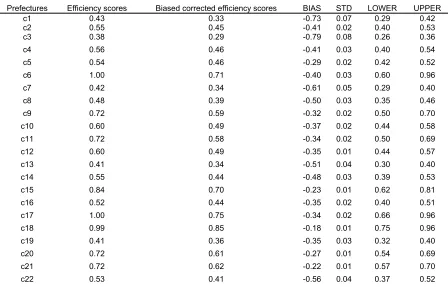
Looking at the results for 1990 (table 4) we realise the Bias is larger than the
standard deviation (std) and therefore the Bias- corrected results have to be preferred
compared to the original estimates. In that respect the five prefectures with the higher
efficiency scores are C18 (THE, 0.85), C37 (ATT, 0.75), C17 (THP, 0.75), C6 (BOI, 0.71)
and C15 (HMA, 0.70). In contrast the five prefectures with the lowest efficiency scores are
C50 (HIO, 0.29), C3 (ARK, 0.29), C28 (LAK, 0.27), C42 (SAM, 0.27) and C31 (LES,
0.25). The mean efficiency scores for 1990 are 0.6 for the original estimates and 0,49 for
[image:18.595.87.535.479.766.2]the Biased –corrected estimates.
Table 4: Efficiency scores, Bias-corrected estimates and confidence internals for 1990 Prefectures Efficiency scores Biased corrected efficiency scores BIAS STD LOWER UPPER
c1 0.43 0.33 -0.73 0.07 0.29 0.42
c2 0.55 0.45 -0.41 0.02 0.40 0.53
c3 0.38 0.29 -0.79 0.08 0.26 0.36
c4 0.56 0.46 -0.41 0.03 0.40 0.54
c5 0.54 0.46 -0.29 0.02 0.42 0.52
c6 1.00 0.71 -0.40 0.03 0.60 0.96
c7 0.42 0.34 -0.61 0.05 0.29 0.40
c8 0.48 0.39 -0.50 0.03 0.35 0.46
c9 0.72 0.59 -0.32 0.02 0.50 0.70
c10 0.60 0.49 -0.37 0.02 0.44 0.58
c11 0.72 0.58 -0.34 0.02 0.50 0.69
c12 0.60 0.49 -0.35 0.01 0.44 0.57
c13 0.41 0.34 -0.51 0.04 0.30 0.40
c14 0.55 0.44 -0.48 0.03 0.39 0.53
c15 0.84 0.70 -0.23 0.01 0.62 0.81
c16 0.52 0.44 -0.35 0.02 0.40 0.51
c17 1.00 0.75 -0.34 0.02 0.66 0.96
c18 0.99 0.85 -0.18 0.01 0.75 0.96
c19 0.41 0.36 -0.35 0.03 0.32 0.40
c20 0.72 0.61 -0.27 0.01 0.54 0.69
c21 0.72 0.62 -0.22 0.01 0.57 0.70
c23 0.56 0.49 -0.28 0.02 0.43 0.54
c24 0.39 0.33 -0.46 0.03 0.30 0.38
c25 0.62 0.53 -0.27 0.01 0.48 0.60
c26 0.65 0.50 -0.45 0.04 0.43 0.62
c27 0.85 0.68 -0.30 0.02 0.58 0.82
c28 0.34 0.27 -0.76 0.11 0.23 0.33
c29 0.66 0.58 -0.21 0.01 0.53 0.64
c30 0.61 0.53 -0.27 0.02 0.46 0.60
c31 0.33 0.25 -0.95 0.15 0.22 0.32
c32 0.46 0.41 -0.26 0.02 0.37 0.45
c33 0.68 0.58 -0.23 0.01 0.52 0.66
c34 0.40 0.33 -0.58 0.04 0.29 0.39
c35 0.60 0.52 -0.27 0.01 0.47 0.58
c36 0.71 0.63 -0.20 0.01 0.57 0.69
c37 1.00 0.75 -0.33 0.01 0.67 0.97
c38 0.64 0.54 -0.27 0.01 0.49 0.61
c39 0.47 0.39 -0.48 0.03 0.34 0.46
c40 0.68 0.59 -0.23 0.01 0.52 0.66
c41 0.78 0.62 -0.34 0.02 0.54 0.75
c42 0.35 0.27 -0.89 0.11 0.24 0.34
c43 0.48 0.41 -0.35 0.03 0.37 0.47
c44 0.64 0.56 -0.21 0.01 0.50 0.62
c45 0.49 0.39 -0.54 0.03 0.35 0.47
c46 0.79 0.62 -0.35 0.02 0.53 0.77
c47 0.52 0.44 -0.37 0.02 0.39 0.51
c48 0.76 0.63 -0.26 0.01 0.56 0.73
c49 0.49 0.42 -0.37 0.02 0.38 0.48
c50 0.37 0.29 -0.72 0.06 0.26 0.36
Mean 0.60 0.49 -0.40 0.03 0.44 0.58
Min 0.33 0.25 -0.95 0.01 0.22 0.32
Std 0.18 0.14 0.18 0.03 0.12 0.17
Finally, looking the efficiency scores of the prefectures for the year 2000 (table 5)
we realise again that the bias is larger than the standard deviation therefore the
Bias-corrected values have to be adopted. The five prefectures with the higher efficiency scores
are: C40 (RET, 0.9), C13 (ZAK, 0.85), C10 (EVR, 0.83), C27 (KYK, 0.77) and C37 (ATT,
0,76). In contrast the five prefectures with the lowest efficiency scores are: C2 (ARG, 0.4),
C7 (GRE/KOZ, 0.33), C4 (ART, 0.32), C8 (DRA, 0.32) and C44 (TRI, 0.32). Finally, the
mean efficiency scores for 2000 are 0.65 for the original estimates and 0.54 for the Biased–
corrected estimates.
Generally, over the last three decades great inefficiencies and efficiency disparities
Greece is reported to have higher efficiency scores (1990, 2000), however prefectures’
welfare efficiencies seem to decrease over the years. This indicates lack of regional policy
implementation among the prefectures’ welfare investments. One of the key elements in
order to improve the welfare state of a prefecture is the account of population density
[image:20.595.96.487.225.773.2]among the years.
Table 5: Efficiency scores, Bias-corrected estimates and confidence internals for 2000
Prefectures
Efficiency
scores Biased corrected efficiency scores BIAS STD LOWER UPPER
c1 0.52 0.44 -0.37 0.02 0.39 0.51
c2 0.51 0.40 -0.56 0.05 0.35 0.50
c3 0.75 0.67 -0.16 0.01 0.60 0.74
c4 0.42 0.32 -0.73 0.08 0.29 0.41
c5 0.66 0.61 -0.13 0.01 0.55 0.65
c6 1.00 0.74 -0.36 0.02 0.63 0.98
c7 0.42 0.33 -0.68 0.06 0.29 0.41
c8 0.42 0.32 -0.74 0.07 0.29 0.41
c9 0.82 0.66 -0.29 0.02 0.58 0.79
c10 0.87 0.83 -0.06 0.00 0.76 0.87
c11 0.69 0.54 -0.39 0.03 0.48 0.66
c12 0.66 0.49 -0.53 0.05 0.42 0.64
c13 1.00 0.85 -0.18 0.01 0.74 0.99
c14 0.62 0.46 -0.53 0.04 0.41 0.60
c15 0.71 0.59 -0.28 0.01 0.54 0.69
c16 0.63 0.50 -0.42 0.02 0.44 0.61
c17 0.57 0.48 -0.31 0.01 0.44 0.55
c18 0.84 0.69 -0.25 0.01 0.62 0.81
c19 0.47 0.41 -0.29 0.02 0.37 0.46
c20 0.52 0.43 -0.39 0.03 0.38 0.50
c21 0.53 0.44 -0.37 0.03 0.39 0.51
c22 0.53 0.42 -0.49 0.04 0.37 0.52
c23 0.57 0.46 -0.40 0.02 0.41 0.55
c24 0.50 0.41 -0.42 0.02 0.37 0.49
c25 0.65 0.60 -0.15 0.01 0.54 0.65
c26 0.92 0.72 -0.30 0.02 0.62 0.89
c27 1.00 0.77 -0.30 0.02 0.67 0.97
c28 0.58 0.53 -0.18 0.01 0.47 0.58
c29 0.68 0.62 -0.15 0.01 0.56 0.67
c30 0.67 0.58 -0.21 0.01 0.53 0.65
c31 0.76 0.71 -0.09 0.00 0.64 0.75
c32 0.51 0.47 -0.16 0.01 0.43 0.51
c33 0.62 0.53 -0.26 0.01 0.48 0.60
c34 0.64 0.58 -0.17 0.01 0.51 0.64
c35 0.56 0.51 -0.20 0.01 0.45 0.55
c36 0.54 0.45 -0.36 0.02 0.41 0.52
c37 1.00 0.76 -0.32 0.02 0.66 0.98
c38 0.57 0.46 -0.42 0.02 0.41 0.55
c39 0.55 0.45 -0.43 0.02 0.40 0.54
c40 1.00 0.90 -0.12 0.00 0.80 0.99
c41 0.55 0.50 -0.21 0.01 0.44 0.55
c43 0.49 0.41 -0.40 0.03 0.36 0.48
c44 0.39 0.32 -0.58 0.06 0.28 0.38
c45 0.68 0.57 -0.30 0.02 0.51 0.66
c46 0.73 0.66 -0.15 0.01 0.60 0.72
c47 0.53 0.42 -0.51 0.04 0.37 0.52
c48 0.61 0.48 -0.45 0.03 0.43 0.59
c49 0.61 0.52 -0.27 0.01 0.47 0.59
c50 0.72 0.68 -0.09 0.00 0.62 0.72
Mean 0.65 0.54 -0.32 0.02 0.48 0.63
Min 0.39 0.32 -0.74 0.00 0.28 0.38
Std 0.17 0.14 0.17 0.02 0.13 0.16
Adopting the methodology proposed by Daraio and Simar [37] we obtained the
[image:21.595.89.485.72.209.2]welfare efficiency scores taking into account the population density of the prefectures.
Table 6 reports the results over the three decades. Again in all the cases the Bias-corrected
estimates are preferred compared to the original efficiency scores. For 1980 the five
prefectures with the higher efficiency scores are C15 (HMA, 0.74), C17 (THP, 0.79), C36
(PEL, 0.68), C37 (ATT, 0.7) and C48 (HAL, 0.69). In contrast the five prefectures with the
lowest efficiency scores are: C47 (FOK, 0.08), C7 (GRE/KOZ, 0.08), C3 (ARK, 0.04), C46
(FLO, 0.02) and C11 (EVI, 0.0014). The mean efficiency scores for 1980 are 0.55 for the
original estimates and 0.46 for the Biased –corrected estimates. In addition for the year
1990 the five prefectures with higher efficiency scores are reported to be: C6 (BOI, 0.74),
C15 (HMA, 0.72), C18 (THE, 0.71), C26 (KOR, 0.71) and C37 (ATT, 0.68). The
prefectures with the lower efficiency scores are reported to be: C8 (DRA, 0.07), C28
(LAK, 0.04), C3 (ARK, 0.03), C47 (FOK, 0.02) and C12 (EVT, 0.01). The mean Biased
corrected efficiency scores for 1990 is 0.44 whereas for the original estimates is 0.54.
Finally, for the year 2000 the five prefectures with the highest efficiency scores are
C6 (BOI, 0.75), C15 (HMA, 0.74), C38 (PIE, 0.74), C9 (DOD, 0.72) and C23 (KER, 0.71).
The prefectures with the lowest efficiency scores are reported to be C8 (DRA, 0.07), C28
(LAK, 0.04), C3 (ARK, 0.04), C12 (EVT, 0.02) and C47 (FOK, 0.02). The mean Biased
results report that over the years the efficiency scores appear to be decreasing over the
years. The evidence provided indicate that there is a decrease of welfare state among the
prefectures over the three census years, indicating (as previously) that there is a lack of
planning on implementing regional welfare investment policies among the prefectures. The
role of population density is a crucial element of welfare provision among the prefectures
[image:22.595.91.534.279.767.2]and its influence on prefectures’ welfare efficiencies needs to be determined.
Table 6: Conditional efficiency scores for the census years of 1980,1990 and 2000
1980 1990 2000
Prefectures θ(x,y)lz θ(x,y)lz cor. θ(x,y)lz θ(x,y)lz cor. θ(x,y)lz θ(x,y)lz cor. c1 0.33 0.28 0.37 0.32 0.23 0.20 c2 0.54 0.46 0.45 0.37 0.41 0.32 c3 0.05 0.04 0.04 0.03 0.04 0.04 c4 0.44 0.38 0.52 0.44 0.38 0.33 c5 0.44 0.39 0.63 0.50 0.84 0.69 c6 0.86 0.71 1.00 0.74 0.98 0.75 c7 0.09 0.08 0.34 0.29 0.30 0.24 c8 0.71 0.60 0.08 0.07 0.08 0.07 c9 0.29 0.25 0.87 0.70 1.00 0.72
c10 0.90 0.83 0.26 0.23 0.26 0.23
c11 0.00 0.00 0.82 0.68 0.53 0.40
c12 0.79 0.65 0.02 0.01 0.02 0.02
c13 0.96 0.82 0.73 0.59 1.00 0.68
c14 0.91 0.76 0.98 0.80 0.72 0.56
c15 1.00 0.74 1.00 0.72 0.95 0.74
c16 0.22 0.20 0.71 0.58 0.89 0.69
c17 1.00 0.79 0.37 0.31 0.08 0.07
c18 0.22 0.18 1.00 0.71 0.90 0.68
c19 0.60 0.52 0.13 0.12 0.13 0.11
c20 0.56 0.47 0.82 0.67 0.59 0.48
c21 0.20 0.18 0.74 0.66 0.35 0.29
c22 0.99 0.83 0.19 0.17 0.18 0.15
c23 0.28 0.25 0.99 0.70 0.90 0.71
c24 0.14 0.12 0.18 0.15 0.29 0.24
c25 0.88 0.74 0.24 0.21 0.19 0.17
c26 0.26 0.22 1.00 0.71 1.00 0.67
c27 0.10 0.09 0.50 0.43 0.61 0.48
c28 0.53 0.46 0.05 0.04 0.05 0.04
c29 0.31 0.27 0.67 0.58 0.56 0.47
c30 0.67 0.58 0.32 0.29 0.30 0.26
c31 0.79 0.70 0.37 0.31 0.55 0.49
c32 0.68 0.57 0.63 0.56 0.49 0.42
c33 0.67 0.55 0.91 0.77 0.79 0.65
c34 0.75 0.66 0.60 0.50 0.52 0.46
c35 0.71 0.62 0.69 0.61 0.53 0.44
c36 1.00 0.68 0.79 0.67 0.56 0.45
c37 1.00 0.70 1.00 0.68 1.00 0.65
c39 0.42 0.35 0.73 0.61 0.69 0.57
c40 0.45 0.41 0.57 0.52 0.75 0.64
c41 0.83 0.75 0.56 0.49 0.29 0.25 c42 0.63 0.57 0.52 0.42 0.46 0.40
c43 0.37 0.33 0.46 0.40 0.37 0.31
c44 0.27 0.24 0.40 0.36 0.17 0.15
c45 0.13 0.11 0.29 0.25 0.28 0.23
c46 0.02 0.02 0.15 0.13 0.08 0.07
c47 0.09 0.08 0.03 0.02 0.03 0.02
c48 1.00 0.69 0.18 0.16 0.15 0.12
c49 1.00 0.78 0.57 0.47 0.66 0.55
c50 0.61 0.55 0.50 0.43 0.69 0.60
Mean 0.55 0.46 0.54 0.44 0.49 0.39
Min 0.00 0.00 0.02 0.01 0.02 0.02
Std 0.32 0.26 0.31 0.24 0.31 0.24
Following, Daraio and Simar [37] figures 2a-c indicate the effect of population
density on prefectures’ welfare efficiencies. For the census year 1980 we realize that the
population density has a moderate effect on welfare efficiencies which can be regarded as
positive. As such population density seem to be taken into account (at least partially) for
1980 and can be regarded that population density plays a role of a “substitutive” input in
the production process, giving the opportunity to “save” inputs in the activity of
production. However, for the census year 1990 and 2000 we realize that the population
density has a clear negative effect on prefectures’ welfare efficiencies and acts like an
“extra” undesired output to be produced asking for the use of more inputs in production
activity [37, p. 105]. It seems that population density fluctuations over the years haven’t
been taken into account when the Greek regional welfare policies have been designed and
implemented. In that respect ‘policy makers must concentrate on regional effects of major
policy strategies rather than on the regional impacts of individual projects or small
programs’ [42, p. 462].
2a
2b
2c
6. Conclusions and Policy Implications
In this study, performing an application of conditional DEA, bootstrap techniques and
kernel density estimations to the Greek prefectures, we obtained, among others, the
efficiency scores and the optimal ratios levels for inefficient prefectures for the census
years of 1980, 1990 and 2000 in terms of their regional welfare policies. In addition this
paper provides a real example of how new advances in DEA methodology as have been
welfare issues and provide a different way for measuring welfare ‘efficiency’. Its unique
advantage for combining multiple criteria into a single measurement provides an excellent
tool for welfare evaluation.
In the case of the Greek prefectures the regional welfare policies are strongly associated
with the regional development and economic efficiency of the particular prefectures. The
efficient prefectures seem to have definite and strong characteristics. Population density
influences negatively Greek prefectures efficiencies, which suggest a lack of regional
welfare investment planning of the regional decision makers. Takahashi [43] suggest that
competition of regional governments that make a decision on the investment in their public
facilities results in an inefficient outcome. Crihfield and McGuire [44] suggest that there is
absence of principles upon which governments can base investment decisions with a direct
impact on regional welfare. These results obtained support the findings of Halkos and
Tzeremes [6] which emphasize major economic inefficiencies among the Greek
prefectures. In addition the results support also the study by Afonso and Fernandes [14]
which indicate that the quantity of the resources of a prefecture doesn’t necessarily ensure
the efficiency of this prefecture if the influence of the external factors (in our case
population density) is not taken into account in regional welfare planning.
On the contrary and in order for a prefecture to attract a certain quantity of resources it
has to develop the appropriate mechanisms to make efficient use of them. Obviously, the
role of governments and policy makers is substantial in stimulating the proper use of the
resources provided by these mechanisms. Moreover, if these mechanisms don’t exist, they
must be created before the recourses are allocated. The policy makers must observe
welfare and regional development as a solid parameter, which eventually has a direct effect
parameters of competition and collaboration with capital spillovers must be taken into
account before any development policy is being applied.
The results indicate that there are policy inefficiencies in terms of welfare among the
Greek prefectures. Furthermore this study supports the study by Karkazis and Thanassoulis
[5] which found significant levels of inefficiencies for Northern Greece indicating policies
inefficiencies and development inequalities among the Greek prefectures. Our results on
regional welfare inefficiencies come to complement the studies by Siriopoulos and
Asteriou [11] and Tsionas [12], which found that there is no real convergence between the
Greek regions, which there is strong evidence of the existence of inefficiencies of welfare
policies among the regions.
Furthermore, the results of our study come along with the suggestions emphasized by
Maudos et al. [13], which indicate that the effort of policy makers must be given to the
improvement of the efficiency of use of productive factors in each sector of activity, rather
than reallocating resources among sectors. Finally, our suggestion to policy makers for the
improvement of regional welfare problems is the adoption of such methodology (and its
new advances) for policy evaluation. Most of the times, its deterministic nature can prove
References
[1] Caminal R. Personal redistribution and the regional allocation of public investment.
Reg Sci Urban Econ 2004; 34: 55-69.
[2] Beer A, Forster C. 2002. Global restructuring, the welfare state and urban programmes:
Federal policies and inequality within Australian cities. Eur Plan Stud 2002; 10: 7-25.
[3] Melachroinos KA, Spence N. Constructing a Manufacturing Fixed Capital Stock Series
for the Regions of Greece. Eur Plan Stud 2000; 8: 43-67.
[4] Aschauer D. Is public expenditure productive? J Monetary Econ 1989; 23: 177–200.
[5] Karkazis J, Thanassoulis Emm. Assessing the effectiveness of regional development
policies in Northern Greece using Data Envelopment Analysis. Soc Econ Plann Sci 1998;
32:123-137.
[6] Halkos GE, Tzeremes NG. Measuring regional economic efficiency: the case of
Greek prefectures. Ann Reg Sci 2009; Doi: 10.1007/s00168-009-0287-6. (article in
press).
[7] Carrera JA, Freire-Seren MJ, Manzano B. Macroeconomic effects of the regional
allocation of public capital formation. Reg Sci Urban Econ 2009; 39: 563-574.
[8] Macmillan WD. The estimation and application of multi-regional economic
planning models using Data Envelopment Analysis. Pap Reg Sci Assoc 1986; 60: 41–
57.
[9] Zhu J. Multidimensional quality-of-life measure with an application to Fortune’s best
cities. Soc Econ Plann Sci 2001; 35:263-284.
[10] Charnes A, Cooper WW, Rhodes EL. Measuring the efficiency of decision making
units. Eur J Oper Res 1978; 2: 429-444.
[11] Siriopoulos C, Asteriou D. Testing for Convergence Across the Greek Regions. Reg
[12] Tsionas EG. Another Look at Regional Convergence in Greece. Reg Stud 2002; 36:
603-609.
[13] Maudos J, Pastor JM, Serrano L. Efficiency and Productive Specialization: An
Application to the Spanish Regions. Reg Stud 2000; 34: 829 – 842.
[14] Afonso A, Fernandes SP. Measuring local government spending efficiency: Evidence
for the Lisbon region. Reg Stud 2006; 40: 39 – 53.
[15] Athanassopoulos AD, Karkazis J. The efficiency of social and economic image
projection in spatial configurations. J Regional Sci 1997; 37:75-97.
[16] De Borger B, Kerstens K, Moesen W, Vanneste J. Explaining differences in
productive efficiency: An application to Belgian municipalities. Public Choice 1994; 80:
339-358.
[17] All Media Database. Profile of Greek Regions. Available from:
http://www.economics.gr. 2007, Accessed 13 Sept 2008.
[18] Boussofiane A, Dyson RG, Thanassoulis E. Applied Data Envelopment Analysis. Eur
J Oper Res 1991; 52:1-15.
[19] Ayres RU. Limits to the growth paradigm. Ecol Econ 1996; 19: 117-134.
[20] Friedly PH. Welfare indicators for public facility investments in urban renewal areas.
Soc Econ Plann Sci 1969; 3: 291-314.
[21] Dyson RG, Allen R, Camanho AS, Podinovski VV, Sarrico CS, Shale E. Pitfalls and
protocols in DEA. Eur J Oper Res 2001; 132: 245-259.
[22] Vogel BW, Coward RT. The Influence of Health and Health Care on Rural Economic
Development. In: Beaulieu LJ, Mulkey D, editors.Investing in People: The Human Capital
[23] Bryden J, Hart K. Dynamics of Rural Areas (DORA): The International Comparison.
Arkleton Centre for Rural Development Research. Aberdeen: University of Aberdeen;
2001.
[24] Cloke P, Phillips M, Thrift N. The new middle classes and the social constructs of
rural living. In: Butler T, Savage M, editors. Social change and the middle classes,
London: UCL Press; 1995.
[25] Bramley G, Smart G. Rural Incomes and Housing Affordability, Salisbury, Wilts:
Rural Development Commission; 1995.
[26] Perroux F. Economic space: Theory and application. Q J Econ 1950; 64:89-104. [27]
Portnov BA, Erell E. Interregional inequalities in Israel, 1948–1995: divergence or
convergence? Soc Econ Plann Sci 2004; 38: 255-289.
[28] Maeda H, Murakami S. Population’s urban environment evaluation model and its
application. J Reg Sci 1985; 25: 273-290.
[29] Shephard RW. Theory of Cost and Production Function. Princeton, NJ: Princeton
University Press; 1970.
[30] Coelli T, Prasada J, Rao DS, Battese GE. An introduction to efficiency and
production analysis. New York: Springer Science; 2005.
[31] Daraio C, Simar L. Advanced robust and nonparametric methods in efficiency
analysis. New York: Springer Science; 2007.
[32] Banker RD, Charnes A, Cooper WW. Some Models for Estimating Technical and
Scale Inefficiencies in Data Envelopment Analysis. Manage Sci 1984; 30:1078– 1092.
[33] Adler N, Yazhemsky E, Tarverdyan R. A framework to measure the relative
socio-economic performance of developing countries. Soc Econ Plann Sci 2010; 44: 73–88.
[34] Simar L, Wilson PW. Sensitivity analysis of efficiency scores: how to bootstrap in
[35] Simar L, Wilson PW. A general methodology for bootstrapping in non-parametric
frontier models. J Appl Stat 2000; 27:779 -802.
[36] Simar L, Wilson PW. Non parametric tests of return to scale. Eur J Oper Res 2002;
139:115-132.
[37] Daraio C, Simar L. Introducing environmental variables in nonparametric frontier
models: A probabilistic approach. J Prod Anal 2005; 24: 93–121.
[38] Simar L, Wilson P. Statistical interference in nonparametric frontier models: recent
developments and perspectives. In: Fried H, Lovell CAK, Schmidt S, editors. The
measurement of productive efficiency and productivity change, New York: Oxford
University Press; 2008.
[39] Silverman BW. Density estimation for statistics and data analysis. London:
Chapman and Hall; 1986.
[40] Nadaraya EA. On estimating regression. Theor Probab Appl 1964; 9:141-142.
[41] Watson GS. Smooth regression analysis. Sankhya Ser A 1964; 26:359-372.
[42] Haveman RH. Evaluating the impact of public policies on regional welfare. Reg
Stud 1976; 10: 449 – 463.
[43] Takahashi T. Spatial competition of governments in the investment on public
facilities. Reg Sci Urban Econ 2004; 34: 455-488.
[44] Crihfield JB, McGuire TJ. Infrastructure, economic development and public
policy. Reg Sci Urban Econ 1997; 27: 113-116.