Simulated annealing least squares twin support vector machine (SA LSTSVM) for pattern classification

Si m ul a t e d a n n e a li n g l e a s t

s q u a r e s t wi n s u p p o r t v e c t o r

m a c hi n e ( SA-L ST SV M) fo r

p a t t e r n cl a s sific a ti o n

S a r t a k h ti, JS, Afr a b a n d p ey, H a n d S a r a e e , M H

h t t p :// dx. d oi.o r g / 1 0 . 1 0 0 7 / s 0 0 5 0 0-0 1 6-2 0 6 7-4

T i t l e

Si m u l a t e d a n n e a li n g l e a s t s q u a r e s t wi n s u p p o r t v e c t o r

m a c h i n e ( SA-LST SV M) fo r p a t t e r n cl a s sific a tio n

A u t h o r s

S a r t a k h ti, JS, Afr a b a n d p ey, H a n d S a r a e e , M H

Typ e

Ar ticl e

U RL

T hi s v e r si o n is a v ail a bl e a t :

h t t p :// u sir. s alfo r d . a c . u k /i d/ e p ri n t/ 3 7 9 5 8 /

P u b l i s h e d D a t e

2 0 1 6

U S IR is a d i gi t al c oll e c ti o n of t h e r e s e a r c h o u t p u t of t h e U n iv e r si ty of S alfo r d .

W h e r e c o p y ri g h t p e r m i t s , f ull t e x t m a t e r i al h el d i n t h e r e p o si t o r y is m a d e

f r e ely a v ail a bl e o nli n e a n d c a n b e r e a d , d o w nl o a d e d a n d c o pi e d fo r n o

n-c o m m e r n-ci al p r iv a t e s t u d y o r r e s e a r n-c h p u r p o s e s . Pl e a s e n-c h e n-c k t h e m a n u s n-c ri p t

fo r a n y f u r t h e r c o p y ri g h t r e s t r i c ti o n s .

F o r m o r e i nfo r m a t io n , in cl u di n g o u r p olicy a n d s u b m i s sio n p r o c e d u r e , p l e a s e

DOI 10.1007/s00500-016-2067-4

M E T H O D O L O G I E S A N D A P P L I C AT I O N

Simulated annealing least squares twin support vector machine

(SA-LSTSVM) for pattern classification

Javad Salimi Sartakhti1 · Homayun Afrabandpey1 · Mohamad Saraee2

© The Author(s) 2016. This article is published with open access at Springerlink.com

Abstract Least squares twin support vector machine (LSTSVM) is a relatively new version of support vector machine (SVM) based on non-parallel twin hyperplanes. Although, LSTSVM is an extremely efficient and fast algo-rithm for binary classification, its parameters depend on the nature of the problem. Problem dependent parameters make the process of tuning the algorithm with best values for parameters very difficult, which affects the accuracy of the algorithm. Simulated annealing (SA) is a random search technique proposed to find the global minimum of a cost function. It works by emulating the process where a metal slowly cooled so that its structure finally “freezes”. This freezing point happens at a minimum energy configuration. The goal of this paper is to improve the accuracy of the LSTSVM algorithm by hybridizing it with simulated anneal-ing. Our research to date suggests that this improvement on the LSTSVM is made for the first time in this paper. Exper-imental results on several benchmark datasets demonstrate that the accuracy of the proposed algorithm is very promis-ing when compared to other classification methods in the literature. In addition, computational time analysis of the algorithm showed the practicality of the proposed algorithm where the computational time of the algorithm falls between LSTSVM and SVM.

Communicated by V. Loia.

B

[email protected]

1 _{Department of Electrical and Computer Engineering (ECE),} Isfahan University of Technology (IUT), 84156-83111 Esfahan, Iran

2 _{School of Computing, Science and Engineering,} University of Salford, Greater Manchester, UK

Keywords Twin support vector machine·Least squares twin support vector machine·Simulated annealing

1 Introduction

Support vector machine (SVM), first introduced byCortes and Vapnik (1995), is a classification technique based on the structural risk minimization (SRM) algorithm. The algo-rithm rapidly became used in many classification tasks due to its success in recognizing handwritten characters in which it outperformed precisely trained neural networks. In addi-tion to recognizing handwritten characters, SVMs performed successful classification in other applications such as: time series prediction (Ruan et al. 2013), pattern classification (Wu et al. 2010), and bioinformatics (Guyon et al. 2002;Sartakhti et al. 2012). A comprehensive tutorial on the SVM classifier algorithm has been published byBurges(1998).

After the introduction of SVM in 1995, different versions of this powerful classifier were advanced including the least squares twin support vector machine (LSTSVM), introduced in 2009 (Arun Kumar and Gopal 2009). LSTSVM combines the idea behind least squares SVM (LSSVM) (Suykens and Vandewalle 1999) and twin SVM (TSVM) (Khemchandani and Chandra 2007).

A crucial challenge in LSTSVM and all other versions of SVM is how to set their parameters with best values. LSTSVM has four parameters which are highly dependent on the nature of the problem. Therefore, finding best val-ues for these parameters is almost impossible for user.Our current research suggests that this is the first study to find the best values for LSTSVM parameters. However, there are several methods for dominating this challenge in SVM.

sev-eral medicine datasets using their proposed GA-based SVM.

Ren and Bai(2010) also presented two approaches for para-meter optimization in SVM, GA-SVM and particle swarm optimization (PSO) SVM. A hybrid ant colony optimiza-tion (ACO) based classifier model which simultaneously optimizes SVM kernel parameters and selects the optimum feature subset has been proposed byHuang(2009). Salimi et al. proposed a method that hybridized SVM and simulated annealing (SA) (Sartakhti et al. 2012). In addition,Lin et al.

(2008) develops a simulated annealing approach for parame-ter deparame-termination and feature selection in the SVM, parame-termed SA-SVM.

Simulated annealing is an optimization algorithm which solves the problem of becoming fixed at local minima (or maxima) by allowing less optimum moves to be chosen sometimes by some probability. The method was described independently by Kirkpatrick et al. (1983) and by Cern`yˇ

(1985). Simulated annealing selects a solution in each iteration by first checking if the neighbor solution is bet-ter than the current solution. If it is, the new solution will be accepted unconditionally. If, however, the neigh-bor solution is not better, it will be accepted based on some probability depending on how much it differs from the neighbor solution and the value of the current solu-tion. In this paper, we have integrated Simulated Annealing with LSTSVM to identify the optimal parameters which enhance LSTSVM accuracy. Our experimental results have demonstrated that the proposed method has higher accura-cies compared to other well-known versions of SVM. In addition, for all evaluated data sets the proposed algorithm outperformed C4.5 which is a powerful algorithm in classi-fication context. Furthermore, computational time analysis showed that our proposed algorithm is faster than SVM and it is completely a practical algorithm for classification tasks.

The rest of this paper is organized as follows. A brief review of basic concepts including SVM and some different versions of the algorithm is presented in Sect.2. The proposed SA-LSTSVM algorithm is introduced in Sect.3. Section4gives the experimental results, and finally in Sect.5conclusions are presented.

2 Basic concepts

This section presents a brief review of different versions of SVM. The versions presented are the standard SVM, TSVM, and LSTSVM.

2.1 Support vector machine

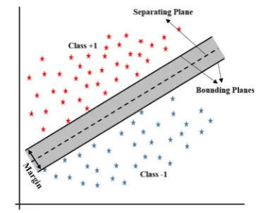
SVM is a maximum margin classifier which means that its goal is to minimize classification error and at the same time

Fig. 1 Geometric interpretation of SVM

maximize the margin between two classes. For example, given a set of training points(xi,yi),i =1, . . . ,neach input

training dataxi ∈ Rd belongs to either of two classes with

labelsyi ∈ −1,+1. SVM seeks a hyperplane with equation

w.x+b=0 which can satisfy the following constraints

yi(w.xi+b)≥1, ∀i. (1)

wherewis the weight vector andbis the bias term. Such a hyperplane could be obtained by solving Eq.2:

Minimize f(x)= w

2

2

subject to yi(w.xi+b)−1≥0 (2)

The geometric interpretation of this formulation is depicted in Fig.1for a toy example.

An important problem with SVM is its computational time. If “l” indicates the size of training data samples, then the computational complexity of SVM is of orderO(l3), which is very expensive.

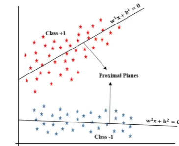
2.2 Twin support vector machine

In SVM only one hyperplane performs the task of partitioning samples into two groups of positive and negative classes. In 2007,Khemchandani and Chandra(2007) proposed TSVM to use two hyperplanes in which samples are assigned to a class according to their distance from each hyperplane. The main equations of TSVM are:

xiw(1)+b(1)=0

xiw(2)+b(2)=0 (3)

wherew(i)andb(i)are weight vectors and bias terms of the

Fig. 2 Geometric interpretations of twin SVM

In TSVM, the two hyperplanes are non-parallel with each being closest to the samples of its own class and farthest from the samples of the opposite class (Ding et al. 2014;

Shao et al. 2011). AssumingAandBindicate data points of class+1 and class−1, respectively, the two hyperplanes are obtained by solving (4) and (5).

Minimize 1 2(Aw

(1)_+e

1b(1))T(Aw(1)+e1b(1))+c1e2Tq

w.r.t. w(1),b(1)

subject to −(Bw(1)+e2b(1))+q ≥e2, q≥0 (4)

Minimize 1 2(Bw

(2)₊

e2b(2))T(Bw(2)+e2b(2))+c2e1Tq

w.r.t. w(2),b(2)

subject to Aw(2)+e1b(2)+q≥e1, q ≥0 (5)

In these equations,qis a vector contains the slack variables,

ei (i ∈ {1,2}) is a column vector of ones with arbitrary

length, andc1andc2are penalty parameters. Once the

hyper-planes are obtained, a new data point is assigned to class+1 or class−1 depending on to which hyperplane the point is closer in terms of perpendicular distance.

In TSVM, the number of constraints in the equation of each hyperplane is equal to the number of samples in the opposite class. Therefore, if there is an equal number of samples in the two classes, the number of constraints for each hyperplane in TSVM is equal to half the number of constraints in SVM. The computational complexity of TSVM is O((l/2)3)(Tomar and Agarwal 2014). It can be shown that the TSVM increases the speed of the algorithm by a factor of 4 compared to the traditional SVM, i.e. it is four times faster when compared to the SVM.

2.3 Least squares twin support vector machine

LSTSVM (Arun Kumar and Gopal 2009;Shao et al. 2012) is a binary classifier which combines the idea of LSSVM (Suykens and Vandewalle 1999; Mitra et al. 2007) and TSVM. LSTSVM employs “least squares of errors” to mod-ify inequality constraints in TSVM to equality constraints by solving a set of linear equations rather than two quadratic pro-gramming problems (QPPs). Experiments have shown that LSTSVM can considerably reduce the training time, while still achieving competitive classification accuracy (Suykens and Vandewalle 1999;Gao et al. 2011). Because LSTSVM is a combination of TSVM and LSSVM, it dramatically reduces the time complexity of SVM. This is because LSTSVM solves equality constraints instead of inequality constraints as in LSSVM which makes the computational speed of the algorithm faster. The number of constraints in each hyper-plane in LSTSVM is half of that in SVM which again results in very low computational complexity when compared to SVM. LSTSVM also has far better accuracy compared to SVM in most classification tasks.

LSTSVM finds its hyperplanes by minimizing Eqs. (6) and (7) which are linearly solvable. By solving (6) and (7), values ofwandbfor each hyperplane are obtained according to (8) and (9).

Minimize 1 2(Aw

(1)₊

eb(1))T(Aw(1)+eb(1))+c1

2q

T

q

w.r.t. w(1),b(1)

subject to (Bw(1)+eb(1))+q =e (6) Minimize 1

2(Bw

(2₎₊

eb(2))T(Bw(2)+eb(2))+c2

2q

T

q

w.r.t. w(2),b(2)

subject to (Aw(2)+eb(2))+q =e (7)

w(1)

b(1)

= −

FTF+ 1 c1

ETE

₋1

FTe (8)

w(2)

b(2)

= −

ETE+ 1 c2

FTF

₋1

ETe (9)

whereE =A eandF =B ewhereasA,B,eandqare introduced in Sect.2.2.

3 Proposed algorithm

LSTSVM has four parameters c1, c2, sigma1 and sigma2

which should be set by the user where c1 and c2

rep-resent the amount of error for each class and sigma1

and sigma2 measure the impact of error on each

nature of the problem which means that for different prob-lems, they would have different optimum values. This affects the accuracy of LSTSVM and is considered as a weakness.

Genetic algorithms, analytical gradient, numerical gradient and Monte Carlo are examples of methods used to find the optimum values for the parameters. Simulated annealing (SA) is also used to find global optimum values for para-meters. Although SA is time consuming, it achieves better accuracies compared to other methods. In this study the SA algorithm is used to find the best global values for LSTSVM parameters.

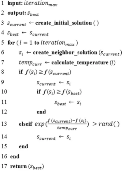
3.1 Simulated annealing

SA is a technique to find the best solution for an optimization problem by trying random variations of the current solution. It is a generalization of a Monte Carlo method for examining equations of state and frozen states ofn-body systems. Figure

3shows the pseudo code of the SA heuristic.

In each step, SA considers some neighboring statesi of the

current statescurrent, and decides between moving to statesi

or staying in statescurrent with some probability. The new

state (si) will be accepted if it has a better fitness compared

to the current state (scurrent). If, however, the new state has

lower fitness, it will be accepted with the probability showed in line 13 of the pseudo code. Note that the definition of

“fit-Fig. 3 Pseudo code of simulated annealing

c= [c1, c2] andsigma= [sigma1, sigma2]

c_←c₀;

sigma←sigma0;

Acc= MyLSTSVM (dataset, classes, method,c0,sigma0);

cbest←c;sigmabest←sigma;Accbest←Acc;

iteration←0;iterationmax←Constant Value (e.g.∞); Whileiteration < iteration_max

{

c_new=c₋0.01 + (0.02)_∗randn(1,2);

sigmanew=sigma−0.0001 + (0.0002)∗randn(1,2);

AccN ew= MyLSTSVM(dataset, classes, method,c₀,sigma₀); ifexp((AccN ew−Acc)∗iteration)> rand(1,1)

{

c_←cnew;sigma_←sigmanew;Acc_←AccN ew;

cbest←cnew;sigmabest←sigmanew;

iteration_←iteration+ 1;

} }

returncbest, sigmabest, Accbest

Fig. 4 Algorithm outline: SA-LSTSVM

ness” depends on the goal of the problem. These probabilistic movements ultimately lead the system to a state with almost optimum solution.

3.2 SA-LSTSVM

This section presents the proposed SA-LSTSVM algorithm in more detail. As already stated, LSTSVM has four parame-ters, two for each of the hyperplanes, which depend on nature of the problem. In SA a set of states is defined where each state has a set of parameters which includec1,c2, sigma1

and sigma2. The start state and its parameters are initiated

by the user. For each state, SA defines a set of neighbors (which are also part of the state set). To find optimum val-ues for LSTSVM parameters, the valval-ues of parameters for each particular state will initially differ from its neighbors. At first, there is a great difference between the parameter val-ues of each two neighbor states, but the difference decreases as the algorithm iterates. In each iteration, a neighbor will be selected randomly. If the selected neighbor has higher accu-racy than the current state, the selected neighbor will be taken and its parameters values (cand sigma) used as new parame-ter values. Figure4shows the pseudo code of the combined algorithm.

4 Experimental results

kmutually exclusive and approximately equal size subsets. Each classification algorithm was trained and testedktimes using these subsets. Each time one of thekfolds is taken as a test set, the remaining(k−1)folds are used as training data. Averaged results of thek-fold cross-validation are con-sidered as the final results. In our evaluation, we used tenfold cross-validation which is a very common case in the context. Furthermore, because simulated annealing tries random vari-ations of the current solution, one may criticize the proposed method that it will be very time consuming for large data sets. To answer this comment, we run our experiments on two types of data sets: small data sets with<2000 samples, and larger data sets with 3000 to 100,000 samples.

4.1 Small data sets

In this section, nine standard small data sets from the UCI repository (Bache and Lichman 2013) were evaluated. Table1shows some features of these data sets.

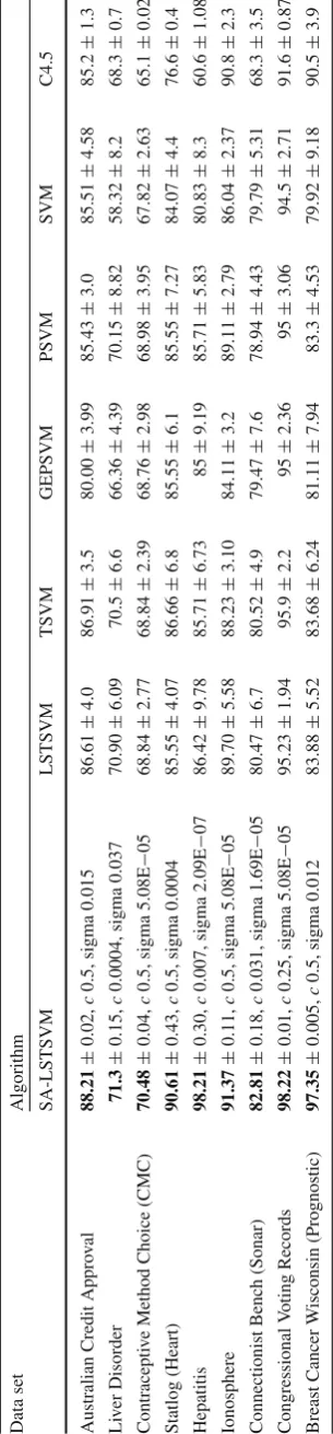
Table2presents the evaluation results of SA-LSTSVM and six other algorithms on these data sets. These algorithms are SVM, four different versions of SVM and a decision tree clas-sification algorithm, C4.5 (Quinlan 1993), which has been selected because of its good performance in classification tasks.Boldtext indicates best accuracies for each data set. In this table the average accuracy of tenfold cross-validation together with the variance of the accuracies are shown as

accuracy±variance. For SA-LSTSVM the best values ofc

and sigma are shown, too. Reported accuracies for TSVM, GEPSVM (Mangasarian and Wild 2006), and PSVM (Fung and Mangasarian 2001) are all extracted fromArun Kumar and Gopal(2009).

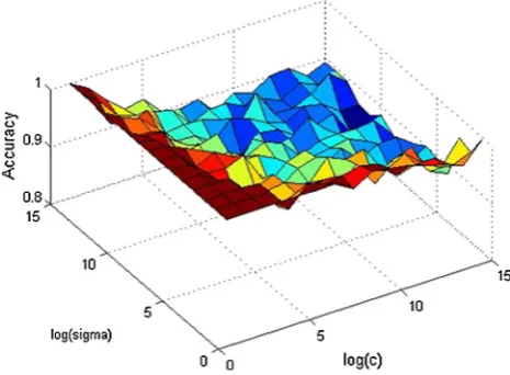
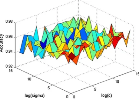
Figures4,5,6,7,8,9,10,11and12show the accuracy of the SA-LSTSVM algorithm for each of the nine data sets for different values ofcand sigma. In some figures, the rela-tion between values of the parameters and the accuracy of SA-LSTSVM is obvious, e.g. Fig.9, however, for some

oth-Table 1 Characteristics of the small data sets

Data sets # features # samples Lost data?

Australian Credit Approval 14 690 No

Liver Disorders 7 345 No

Contraceptive Method Choice (CMC)

9 1473 No

Statlog (Heart) 13 270 No

Hepatitis 19 155 Yes

Ionosphere 34 351 No

Connectionist Bench (Sonar) 60 208 No

Congressional Voting Records 16 435 Yes Breast Cancer Wisconsin

(Prognostic)

34 198 No

Fig. 5 Changes in the accuracy of SA-LSTSVM for different values ofcand sigma on Australian Credit Approval data set

Fig. 6 Changes in the accuracy of SA-LSTSVM for different values ofcand sigma on Liver Disorder data set

Fig. 7 Changes in the accuracy of SA-LSTSVM for different values ofcand sigma on CMC data set

ers, e.g. Fig.7there is not an obvious relationship between the accuracy of SA-LSTSVM and values of the parameters. As it is mentioned before the optimum values for

parame-Fig. 8 Changes in the accuracy of SA-LSTSVM for different values ofcand sigma on Statlog (Heart) data set

Fig. 9 Changes in the accuracy of SA-LSTSVM for different values ofcand sigma on Hepatitis data set

Fig. 10 Changes in the accuracy of SA-LSTSVM for different values ofcand sigma on Ionosphere data set

Fig. 11 Changes in the accuracy of SA-LSTSVM for different values ofcand sigma on Sonar data set

Fig. 12 Changes in the accuracy of SA-LSTSVM for different values ofcand sigma on Congressional Voting Records data set

Fig. 13 Changes in the accuracy of SA-LSTSVM for different values ofcand sigma on Breast Cancer Wisconsin data set

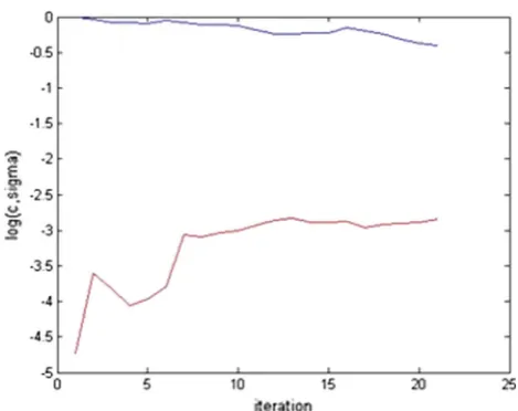
Figures13,14,15,16,17,18,19,20and21show how the values ofcand sigma changed during iterations of the SA algorithm for the nine data sets. In these figures, the blue

Fig. 14 Changes ofcand sigma in SA-LSTSVM on Australian Credit Approval data set

Fig. 15 Changes ofcand sigma in SA-LSTSVM on Liver Disorder data set

Fig. 17 Changes ofcand sigma in SA-LSTSVM on Statlog (Heart) data set

Fig. 18 Changes ofcand sigma in SA-LSTSVM on Hepatitis data set

Fig. 19 Changes ofcand sigma in SA-LSTSVM on Ionosphere data set

Fig. 20 Changes ofcand sigma in SA-LSTSVM on Sonar data set

Fig. 21 Changes ofcand sigma in SA-LSTSVM on Congressional Voting Records data set

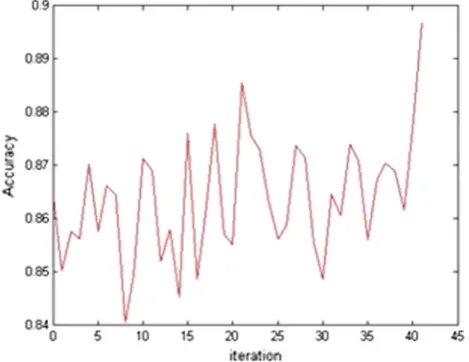
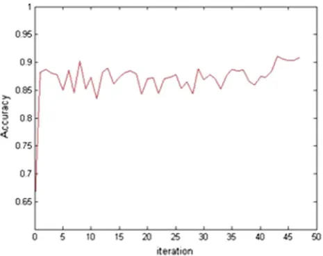
shows the changes in the value ofcand the red curve shows how sigma changes during the iterations. As it can be seen from the figures, the way the algorithm moves toward the optimum values for parameters depends on the data set. Figures22,23,24,25,26,27,28,29,30and31show how the accuracy of the SA-LSTSVM algorithm changes during iterations of SA algorithm on the data sets. The figures show that as the algorithm iterates the average accuracy increases, but the accuracy variances decreased. The figures also show that using SA-LSTSVM it is possible to achieve the global best accuracy in a limited number of iterations (<60 iteration in most of the data sets).

4.2 Larger data sets

Musi-Fig. 22 Changes ofcand sigma in SA-LSTSVM on Breast Cancer Wisconsin data set

Fig. 23 Changes of the accuracy of SA-LSTSVM on Australian Credit Approval data set

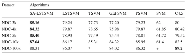
cant 1998) to generate data sets with 3000, 4000, 5000, 10,000, and 100,000 samples and 32 features. Results of run-ning each algorithm are shown in Table3. The best accuracy for each data set is shown inboldface. As it is shown in the table, again SA-LSTSVM has the highest accuracies among all versions of SVM for all data sets. However, only in NDC-100k data set, C4.5 obtains a better accuracy compared to SA-LSTSVM.

4.3 Statistical comparison of classifiers

The above experiments showed that for all of the studied datasets, the accuracy of SA-LSTSVM is higher than other compared algorithms. However, there still a question remains which is “Are these differences statistically significant?”. In other words, it is important to show that these algorithms are

Fig. 24 Changes of the accuracy of SA-LSTSVM on Liver Disorder data set

Fig. 25 Changes of the accuracy of SA-LSTSVM on CMC data set

Fig. 27 Changes of the accuracy of SA-LSTSVM on Hepatitis data set

Fig. 28 Changes of the accuracy of SA-LSTSVM on Ionosphere data set

Fig. 29 Changes of the accuracy of SA-LSTSVM on Sonar data set

Fig. 30 Changes of the accuracy of SA-LSTSVM on Congressional Voting Records data set

Fig. 31 Changes of the accuracy of SA-LSTSVM on Breast Cancer Wisconsin data set

statistically different. InDemšar(2006), Demsar introduced different ways of comparing algorithms over multiple data sets. Since we have seven algorithms for comparison, we choose to use Friedman test which is a non-parametric coun-terpart of ANOVA. Although there are some implementations of the Friedman test in some software tools like MATLAB and KEEL (Alcal-Fdez et al. 2009), we chose to implement the test by ourselves in MATLAB. The Friedman test ranks the algorithms for each dataset separately in the way that the best performing algorithm getting the rank 1, the second best ranked 2 and so on. In case of ties, e.g. in CMC, Hepati-tis, Congressional Voting Records, and NDC-4k, the average ranks are assigned. Table4shows the ranks of the classifiers for different datasets used in this paper. Numbers inside the parenthesis are the ranks of classifiers for the correspond-ing dataset. The final row contains the average ranks of each classifier which is computed as Rj = 1

Table 3 Experimental results of SA-LSTSVM and other algorithms on larger data sets

Dataset Algorithms

SA-LSTSVM LSTSVM TSVM GEPSVM PSVM SVM C4.5

NDC-3k 85.16 79.24 77.73 77.20 79.23 62 80

NDC-4k 84.32 79.87 78.65 75.98 79.87 61.85 80.42

NDC-5k 85.40 78.93 77.49 75.43 78.01 61.72 79.52

NDC-10k 87.64 86.17 85.31 84.32 85.95 61.4 82.5

NDC-100k 88.31 86.07 * 84.02 86.32 ∗ 89.2

The∗sign shows that the algorithm did not converge in a reasonable time

Table 4 Rankings of the classifiers for each dataset

Dataset Algorithms

SA-LSTSVM LSTSVM TSVM GEPSVM PSVM SVM C4.5

Australian Credit Approval 88.21(1) 86.61 (3) 86.91 (2) 80.00 (7) 85.43 (5) 85.51 (4) 85.2 (6)

Liver Disorder 71.3(1) 70.90 (2) 70.5 (3) 66.36 (6) 70.15 (4) 58.32 (7) 68.3 (5)

Contraceptive Method Choice (CMC) 70.48(1) 68.84 (3.5) 68.84 (3.5) 68.76 (5) 68.98 (2) 67.82 (6) 65.1 (7)

Statlog (Heart) 90.61(1) 85.55 (4) 86.66 (2) 85.55 (4) 85.55 (4) 84.07 (6) 76.6 (7)

Hepatitis 98.21(1) 86.42 (2) 85.71 (3.5) 85 (5) 85.71 (3.5) 80.83 (6) 60.6 (7)

Ionosphere 91.37(1) 89.70 (3) 88.23 (5) 84.11 (7) 89.11 (4) 86.04 (6) 90.8 (2)

Connectionist Bench (Sonar) 82.81(1) 80.47 (3) 80.52 (2) 79.47 (5) 78.94 (6) 79.79 (4) 68.3 (7) Congressional Voting Records 98.22(1) 95.23 (3) 95.9 (2) 95 (4.5) 95 (4.5) 94.5 (6) 91.6 (7) Breast Cancer Wisconsin (Prognostic) 97.35(1) 83.88 (3) 83.68 (4) 81.11 (6) 83.3 (5) 79.92 (7) 90.5 (2)

NDC-3k 85.16(1) 79.24 (3) 77.73 (5) 77.20 (6) 79.23 (4) 62 (7) 80 (2)

NDC-4k 84.32(1) 79.87 (3.5) 78.65 (5) 75.98 (6) 79.87 (3.5) 61.85 (7) 80.42 (2)

NDC-5k 85.40(1) 78.93 (3) 77.49 (5) 75.43 (6) 78.01 (4) 61.72 (7) 79.52 (2)

NDC-10k 87.64(1) 86.17 (2) 85.31 (4) 84.32 (5) 85.95 (3) 61.4 (7) 82.5 (6)

Average Rank 1 2.923 3.538 5.576 4.038 6.153 4.769

is the rank of thejth algorithm on theith dataset. Note that since for NDC-100k two of the algorithms do not converged, we do not count this dataset in the evaluation.

The above experiments showed that for all of the studied datasets, the accuracy of SA-LSTSVM is higher than other compared algorithms. However, there still a question remains which is “Are these differences statistically significant?”. In other words, it is important to show that these algorithms are statistically different. InDemšar(2006), Demsar introduced different ways of comparing algorithms over multiple data sets. Since we have seven algorithms for comparison, we choose to use Friedman test which is a non-parametric coun-terpart of ANOVA. Although there are some implementations of the Friedman test in some software tools like MATLAB and KEEL (Alcal-Fdez et al. 2009), we chose to implement the test by ourselves in MATLAB. The Friedman test ranks the algorithms for each dataset separately in the way that the best performing algorithm getting the rank 1, the second best ranked 2 and so on. In case of ties, e.g. in CMC, Hepati-tis, Congressional Voting Records, and NDC-4k, the average ranks are assigned. Table4shows the ranks of the classifiers for different datasets used in this paper. Numbers inside the

parenthesis are the ranks of classifiers for the correspond-ing dataset. The final row contains the average ranks of each classifier which is computed as Rj = _N1

ir j

i, wherer j i

is the rank of thejth algorithm on theith dataset. Note that since for NDC-100k two of the algorithms do not converged, we do not count this dataset in the evaluation.

The null-hypothesis is that all the algorithms are equiva-lent. Then the Friedman statistic is calculated and finally the critical value of the distribution of the Friedman statistic is compared with the statistic itself. The null-hypothesis will be rejected if the statistic is higher than the critical value. The Friedman statistic is computed as follows:

χ2

F =

12N k(k+1)

⎡ ⎣

j

R2j−

k(k+1)2 4

⎤

⎦_. (10)

In this equation,kandNare the total number of classifiers and the total number of datasets, respectively. In our case

k =7 and N =13. The statistic is distributed according to

χ2

F withk−1 degrees of freedom, when N andk are big

case (Demšar 2006).Iman and Davenport(1980) showed that Friedman’sχ_F2is undesirably conservative and they proposed a better statistic as bellow.

FF= (

N−1)χ_F2

N(k−1)−χ_F2 (11)

which is distributed according to theF-distribution withk−1 and(k−1)(N−1)degrees of freedom.

The computed Friedman statistic and the correspondingFF

statistic for our experiments are:

χ2

F =

12∗13 7∗8

(12+2.9232+3.5382+5.5762

+4.0382+6.1532+4.7692)−7∗8

2

4

=50.3

FF=

12∗50.3

13∗6−50.3 =21.8

With seven algorithms and 13 datasets, FF is distributed

according to the F distribution with 7−1 = 6 and(7− 1)×(13−1)=72 degrees of freedom. The critical value of F(6,72) for α = 0.05 is 2.23, so we reject the null-hypothesis which means that the algorithms are statistically different.

By rejecting the null-hypothesis we can proceed with a post-hoc test. Since we want to compare all other classifiers with our proposed SA-LSTSVM, we will use the Bonferroni– Dunn test (Dunn 1961). InDemšar(2006) it is explained that based on Nemenyi test (Nemenyi 1963), the performance of two classifiers is significantly different if the corresponding average ranks differ by at least the critical difference CD=q_α

k(k+1) 6N

whereqα is the critical value.

The Bonferroni–Dunn test controls the family wise error rate by divingαby the number of comparisons made which is

k−1 in this case. The alternative way to compute the same test as it is introduced inDemšar(2006) is to compute the critical difference, CD, using the same equation as the Nemenyi test, but using the critical values for_(k−α₁₎. The critical valueq0_.05

for seven classifiers is 2.638 and, therefore, we have CD

=2.638

7∗8

6∗13 =2.235. Using this critical difference, we

can conclude that:

• SA-LSTSVM performs significantly better that LSTSVM, since 1−2.923<2.235

• SA-LSTSVM performs significantly better that TSVM, since 1−3.538<2.235

• SA-LSTSVM performs significantly better that GEPSVM, since 1−5.576<2.235

Table 5 Computational time analysis (in second) of SVM, LSTSVM and SA-LSTSVM

Data sets Algorithms SVM LSTSVM SA-LSTSVM

Australian Credit Approval 1.9 0.014 1.74 Liver Disorder 1.85 0.008 1.01 Contraceptive Method

Choice (CMC)

3.6 0.018 0.87

Statlog (Heart) 1.58 0.013 1.11

Hepatitis 1.3 0.009 0.93

Ionosphere 1.49 0.035 0.69

Connectionist Bench (Sonar)

1.45 0.053 1.29

Congressional Voting Records

3.21 0.008 1.6

Breast Cancer Wisconsin (Prognostic)

3.73 0.028 0.8

NDC-3k 11.08 0.009 3.05

NDC-4k 22.83 0.014 7.54

NDC-5k 59.58 0.018 45.50

NDC-10k 241.68 0.026 211.56

NDC-100k ∗ 0.19 1684.82

• SA-LSTSVM performs significantly better that PSVM, since 1−4.038<2.235

• SA-LSTSVM performs significantly better that SVM, since 1−6.153<2.235

• SA-LSTSVM performs significantly better that C4.5, since 1−4.769<2.235.

4.4 Computational time analysis

As stated in Sect.2.3, LSTSVM is computationally faster than SVM with a computational time better than SVM by a factor of 4. SA is a probabilistic meta heuristic algorithm which takes random walks through the problem space. This may suggest that the SA-LSTSVM algorithm may be com-putationally very slow. However, our computational time analysis indicates otherwise.

Table5shows the computational times in second for the SA-LSTSVM, LSTSVM and SVM algorithm for all of the data sets. For the SA-LSTSVM algorithm the maximum number of iterations considered in the experiment was 25. This num-ber was chosen because with this value forkmax, the algorithm

com-putational times for LSTSVM are better than SA-LSTSVM and SVM, the proposed SA-LSTSVM has higher accura-cies when compared to both LSTSVM and SVM for all data sets.

5 Conclusion

The LSTSVM algorithm is a relatively new addition of the family of SVM classifier algorithms and being based on non-parallel twin hyperplanes has shown good classifica-tion performance. However, the algorithm has parameters which are problem dependent and finding the optimum val-ues for these parameters is itself a challenging problem that affects the accuracy of the algorithm. In this paper we have proposed an improved LSTSVM algorithm (SA-LSTSVM) by hybridizing it with the well-known simulated annealing (SA) algorithm to determine the optimum parameter values for the LSTSVM algorithm. Experimental results on data sets with different sizes have demonstrated that the algo-rithm has higher accuracies compared to other well-known classification algorithms while its computational time is also reasonable.

Compliance with ethical standards

Conflict of interest The authors declare that they have no conflict of interest.

Open Access This article is distributed under the terms of the Creative Commons Attribution 4.0 International License (http://creativecomm ons.org/licenses/by/4.0/), which permits unrestricted use, distribution, and reproduction in any medium, provided you give appropriate credit to the original author(s) and the source, provide a link to the Creative Commons license, and indicate if changes were made.

References

Alcal-Fdez J, Snchez L, Garca S, del Jesus M, Ventura S, Garrell J, Otero J, Romero C, Bacardit J, Rivas V, Fernndez J, Herrera F (2009) Keel: a software tool to assess evolutionary algorithms for data mining problems. Soft Comput 13(3):307–318

Arun Kumar M, Gopal M (2009) Least squares twin support vector machines for pattern classification. Expert Syst Appl 36(4):7535– 7543

Bache K, Lichman M (2013) UCI machine learning repository.http:// archive.ics.uci.edu/ml

Burges CJ (1998) A tutorial on support vector machines for pattern recognition. Data Min Knowl Discov 2(2):121–167

ˇ

Cern`y V (1985) Thermodynamical approach to the traveling salesman problem: an efficient simulation algorithm. J Optim Theory Appl 45(1):41–51

Cortes C, Vapnik V (1995) Support-vector networks. Mach Learn 20(3):273–297

Delen D, Walker G, Kadam A (2005) Predicting breast cancer surviv-ability: a comparison of three data mining methods. Artif Intell Med 34(2):113–127

Demšar J (2006) Statistical comparisons of classifiers over multiple data sets. J Mach Learn Res 7:1–30

Ding S, Yu J, Qi B, Huang H (2014) An overview on twin support vector machines. Artif Intell Rev 42(2):245–252

Dunn OJ (1961) Multiple comparisons among means. J Am Stat Assoc 56(293):52–64

Fung G, Mangasarian OL (2001) Proximal support vector machine clas-sifiers. In: Proceedings of the seventh ACM SIGKDD international conference on knowledge discovery and data mining. ACM, New York, pp 77–86

Gao S, Ye Q, Ye N (2011) 1-norm least squares twin support vector machines. Neurocomputing 74(17):3590–3597

Guyon I, Weston J, Barnhill S, Vapnik V (2002) Gene selection for cancer classification using support vector machines. Mach Learn 46(1–3):389–422

Huang C-L (2009) ACO-based hybrid classification system with feature subset selection and model parameters optimization. Neurocom-puting 73(1):438–448

Huang C-L, Wang C-J (2006) A GA-based feature selection and para-meters optimizationfor support vector machines. Expert Syst Appl 31(2):231–240

Iman RL, Davenport JM (1980) Approximations of the critical region of the Fbietkan statistic. Commun Stat Theory Methods 9(6):571– 595

Khemchandani R, Chandra S et al (2007) Twin support vector machines for pattern classification. IEEE Trans Pattern Anal Mach Intell 29(5):905–910

Kirkpatrick S, Gelatt CD, Vecchi MP (1983) Optimization by simulated annealing. Science 220(4598):671–680

Lin S-W, Lee Z-J, Chen S-C, Tseng T-Y (2008) Parameter determination of support vector machine and feature selection using simulated annealing approach. Appl Soft Comput 8(4):1505–1512 Mangasarian OL, Wild EW (2006) Multisurface proximal support

vec-tor machine classification via generalized eigenvalues. IEEE Trans Pattern Anal Mach Intell 28(1):69–74

Mitra V, Wang C-J, Banerjee S (2007) Text classification: a least square support vector machine approach. Appl Soft Comput 7(3):908– 914

Musicant DR (1998) NDC: normally distributed clustered datasets.

http://www.cs.wisc.edu/dmi/svm/ndc/

Nemenyi P (1963) Distribution-free multiple comparisons. https:// books.google.fi/books?id=nhDMtgAACAAJ

Quinlan JR (1993) C4. 5: programs for machine learning, vol 1. Morgan Kaufmann, Burlington

Ren Y, Bai G (2010) Determination of optimal SVM parameters by using GA/PSO. J Comput 5(8):1160–1168

Ruan J, Wang X, Shi Y (2013) Developing fast predictors for large-scale time series using fuzzy granular support vector machines. Appl Soft Comput 13(9):3981–4000

Sartakhti JS, Zangooei MH, Mozafari K (2012) Hepatitis disease diag-nosis using a novel hybrid method based on support vector machine and simulated annealing (svm-sa). Comput Methods Progr Biomed 108(2):570–579

Shao Y-H, Zhang C-H, Wang X-B, Deng N-Y (2011) Improvements on twin support vector machines. IEEE Trans Neural Netw 22(6):962–968

Shao Y-H, Deng N-Y, Yang Z-M (2012) Least squares recursive pro-jection twin support vector machine for classification. Pattern Recognit 45(6):2299–2307

Suykens JA, Vandewalle J (1999) Least squares support vector machine classifiers. Neural Process Lett 9(3):293–300

Tomar D, Agarwal S (2014) Feature selection based least square twin support vector machine for diagnosis of heart disease. Int J Bio Sci Bio Technol 6(2)