Lossless Image Compression Using Neural Network

(1)

International Journal of Emerging Technology and Advanced Engineering

Website: www.ijetae.com (ISSN 2250-2459,ISO 9001:2008 Certified Journal, Volume 5, Issue 6, June 2015)

231

Lossless Image Compression Using Neural Network

Aakash Niras

1

, Gaurav Ojha

2

Sanjay Sachan

3

1,2_{Research Scholar, AIET Lucknow, India} 3_{Head IT Dept, AIET Lucknow, India}

Abstract- Image Compression and Data compression has

always been a great challenge and thus provide greater opportunities for exploration. The original image acquires a considerable space on disk and it is not network friendly as well to be transferred over internet. It needs to be reduced in disk size reducing storage space as well as making it easier to be transferred on the network. In this paper an investigation has been done with possibilities of using neural network for image compression. Various algorithms have been tried and tested with a number of test images to find the most suitable out of them. The various learning methods like quasi newton method, LM method, Gradient descent method have been used to perform the training of the network architecture and finally the performance of these is evaluated in terms of MSE

and PSNR.

Index Terms- Lossy and Lossless Image Compression,

Artificial Neural Network, Bipolar Backpropagation coding Technique, Levenberg-Marquardt (LM) Algorithm, Quasi-Newton method, Gradient descent method, Peak Signal to Noise Ratio, PCA Technique, Error vs. Epochs Graphs.

I. INTRODUCTION

Uncompressed multimedia (graphics, audio and video)

data requires considerable storage capacity and

transmission bandwidth. Despite rapid progress in

mass-storage density, processor speeds, and digital

communication system performance, demand for data

storage capacity and data-transmission bandwidth

continues to outstrip the capabilities of available technologies.

The main aim of image compression is to remove the redundancy from image in so as to allow the same image reconstruction at the receiver end. There are mainly two types of image compression techniques, lossy and lossless. In medical applications, the images are compressed by lossless compression methods because each bit of information is important. The digital or video image data are compressed by lossy compression techniques where certain bits can be skipped without much affecting the quality of the data.[1-3]. For such type of compression, transform coding techniques like cosine transform, wavelet transform are very effective techniques, which give better results but it process the data in serial manner and hence requires more time for processing [4].

The artificial neural network is a recent tool in image compression as it processes the data in parallel and hence requires less time and therefore, it is superior over any other technique.

The paper consists of 8 sections. Section 2 describes the basic Artificial Neural network structure. Section 3 gives the information about the training algorithm used section 4 explains the bipolar back propagation coding technique. The various learning algorithms have been discussed in Section 5. Section 6 caters to Performance parameters, Results and discussion are presented in Section 7. Finally, section 8 presents the conclusion and future work.

II. ARTIFICIAL NEURAL NETWORK

An Artificial Neural Network is a parallel processing system which is better than linear computing method. ANN is mathematical model which is modeled according the human being nervous system, such as brain process system.. Another function computes the output of the

neurons.

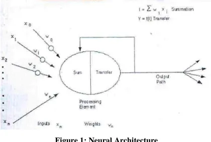
The basic unit of neural networks, the

[image:1.612.338.548.501.643.2]

artificial neurons, simulates the four basic functions

of natural neurons. Artificial neurons are much

simpler than the biological neuron; the figure below

shows the basics of an artificial neuron.

Figure 1: Neural Architecture

A neural network architecture as shown in Figure 2 for solving the image compression problem.

(2)

International Journal of Emerging Technology and Advanced Engineering

232 One of the most important types of feed forward network is the multilayer back propagation neural network [9,10].

[image:2.612.82.255.184.306.2]

Figure 2 Learning Neurons

The input layer consists of neurons that receive input form the external environment. The output layer consists of neurons that communicate the output of the system to the user or external environment. There are usually a number of hidden layers between these two layers; the figure below shows a simple structure with only one hidden layer.

[image:2.612.89.258.410.542.2]

Figure 3: Three Perceptron Model

When the input layer receives the input its neurons produce output, which becomes input to the other layers of the system. The process continues until a certain condition is satisfied or until layer is invoked and fires their output to the external environment.

The neural network architecture for image compression designed here consists of here 64 input neurons, 16 hidden neurons and 64 output neurons according to the requirements. The input layer encodes the inputs of neurons and transmits the information to the hidden layer of neurons. The out put layer receives the hidden layer information and decodes the information according to the function used at the output.

The outputs of hidden layer are real valued and require large number of bits to transmit the data. The transmitter encodes and then transmits the output of the hidden layer 16 values as compared to the 64 values of the original image. The receiver receives and decodes the 16 hidden neurons output and generates 64 outputs neurons at the output layer.

III. BIPOLAR BACK PROPAGATION CODING

TECHNIQUE

The image pixels in the image data firstly needs to be normalized so as to reduce the data range and reduce the complexity for the neural network input. The desired range of data values for the input at the entry layer of neural network should lie between 0 to1 so that the input layer can easily assign a binary code with these values. At the output layer this needs to be converted back to the original form in the form of pixels before constructing it as image.

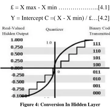
The compression and quality of image depends on number of neurons present in the hidden layer. The quality of output image improves and the data loss reduces as the number of hidden neurons increases. The conversions are based on certain ranges where analog form is scaled between value 0 and 1. Thus, for converting analog values into digital form, different binary values can be assigned. In this technique, each value is converted into the range between 0 and 1 using the formula as follows [1-2]

£ = X max - X min ………..[4.1]

Y = Intercept C =( X - X min) / £…[4.2]

Figure 4: Conversion In Hidden Layer

[image:2.612.345.526.450.626.2]

(3)

International Journal of Emerging Technology and Advanced Engineering

233 The above figure shows the algorithm used for implementing the proposed technique. „Purelin‟ and „tansig‟ transfer functions are used at the input layer and the hidden layers respectively to train the neurons. The neurons are trained used different learning algorithms viz. Lavenberg Marquardt algorithm, quasi-newton method and gradient descent methods for an error limit of 10-5. Once the neurons are trained the image to be compressed is given to the trained network and the resultant output is found to be compressed in disk size.

The performance of different training algorithm is evaluated and compared on different parameters like Mean square Error (MSE) and PSNR.

IV. LEARNING ALGORITHMS

A learning rule is defined as a procedure for modifying the weights and biases of a network. The learning rule is applied to train the network to perform some particular task. Learning rules fall into two broad categories: supervised learning, and unsupervised learning[16-17].

In supervised learning, the learning rule is provided with a set of examples (the training set) of proper network behavior

Where is an input to the network, and is the corresponding correct (target) output. As the inputs are applied to the network, the network outputs are compared to the targets.

The learning rule is then used to adjust the weights and biases of the network in order to move the network outputs closer to the targets. The perceptron learning rule falls in this supervised learning category.

In unsupervised learning, the weights and biases are modified in response to network inputs only. There are no target outputs available. Most of these algorithms perform clustering operations. They categorize the input patterns into a finite number of classes. This is especially useful in such applications as vector quantization.

Backpropagation Training Algorithms:

Gradient Descent: There are many variations of the backpropagation algorithm. The simplest implementation of backpropagation learning updates the network weights and biases in the direction in which the performance function decreases most rapidly, the negative of the gradient. One iteration of this algorithm can be written

Where is a vector of current weights and biases, is the current gradient, and is the learning rate. There are two different ways in which this gradient descent algorithm can be implemented: incremental mode and batch mode. In incremental mode, the gradient is computed and the weights are updated after each input is applied to the network. In batch mode, all the inputs are applied to the network before the weights are updated.

BFGS Algorithm: Newton's method is an alternative to the conjugate gradient methods for fast optimization[16-17]. The basic step of Newton's method is

(4)

International Journal of Emerging Technology and Advanced Engineering

234 Levenberg-Marquardt: Like the quasi-Newton methods, the Levenberg Marquardt algorithm was designed to approach second-order training speed without having to compute the Hessian matrix. When the performance function has the form of a sum of squares, then the Hessian matrix can be approximated as:

And the gradient can be computed as:

Where J is the Jacobian matrix that contains first derivatives of the network errors with respect to the weights and biases, and e is a vector of network errors. The Jacobian matrix can be computed through a standard back-propagation technique that is much less complex than computing the Hessian matrix.

The Levenberg-Marquardt algorithm uses this

approximation to the Hessian matrix in the following Newton-like update[17]:

V. PERFORMANCE PARAMETERS

The parameters like Mean Square Error (MSE) and Peak Signal to Noise ratio (PSNR) are generally used to measure the quality of an image. MSE and PSNR are those parameters that define the quality of an image reconstructed at the output layer of neural network architecture. The MSE between the target image and reconstructed image should be very small, almost negligible so that the quality of reconstructed image should be nearly same to the target image. Ideally, MSE should be zero for ideal decompression. The error is evaluated by comparing the input image and decompressed image using normalized mean square error formula [13].

Where is the target value and is the output of the neural network.

An alternative to MSE, the quality of decompressed image can also be expressed in terms of peak signal to noise ratio (PSNR) is also introduced which is defined as[14]:

Where L is the maximum value of pixels of an image.

VI. RESULT AND SIMULATION

The above algorithms have been tested using MATLAB R2010a version. MATLAB has dedicated functions package for Neural Network, thus the algorithms has been implemented using this toolbox functions.

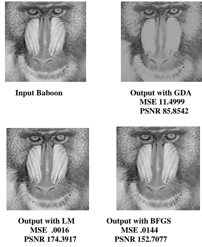
Different test images were taken for the experiment. Each image was of 256x256 pixels size in png format. The three algorithms viz. gradient descent, Lavenberg-Marquardt and quasi newton have been applied and the results and output compressed image are derived as shown below:

Input Baboon Output with GDA MSE 11.4999 PSNR 85.8542

[image:4.612.340.543.385.634.2]

Output with LM Output with BFGS MSE .0016 MSE .0144 PSNR 174.3917 PSNR 152.7077

(5)

International Journal of Emerging Technology and Advanced Engineering

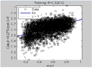
[image:5.612.72.264.134.275.2] [image:5.612.73.265.292.472.2]

235 Figure 7: Regression plot GDA Algorithm

[image:5.612.71.264.413.634.2]

Figure 8:Regression Plot BFGS Algorithm

Figure 9: Regression plot LM Algorithm

VII. CONCLUSION AND FUTURE WORK

This paper takes investigates into novice prospective of image compression using Neural Network Architectures.

The various different kinds of training algorithms were applied on a set of test images and there results were compared on various performance parameters viz. MSE, PSNR, Regression plots as well as the quality of the output image. LM Algorithm and BFGS Algorithm gave good results in terms of image quality and PSNR but the time taken in implementation of LM Algorithm was considerably less than the BFGS Algorithm. Thus the possibilities of using this training method and Neural Network are immense as the size of most of the images has been reduced to less than half. The author can clearly visualize the importance of this technique in the future of Image Processing on various other aspects apart from Image Compression like Image Segmentation Denoising etc.

REFRENCES

[1] E. Watanabe and K. Mori, “Lossy Image Compression Using a Modular Structured Neural Network,” Proceed- ings of IEEE Signal Processing Society Workshop, Wash- ington DC, 2001, pp. 403-412. [2] M. J. Weinberger, G. Seroussi and G. Sapiro, “The LOCO-I Lossless Image Compression Algorithm: Principles and Sta- ndardization into JPEG-LS,” IEEE Transaction on Image Processing, Vol. 9, No. 8, 2000, pp. 1309-1324.

[3] V. H. Gaidhane, Y. V. Hote and V. Singh, “A New Ap-proach for Estimation of Eigenvalues of Images,” Inter- national Journal of Computer Applications, Vol. 26, No. 9, 2011, pp. 1-6.

[4] S.-G. Miaou and C.-L. Lin, “A Quality-on-Demand Algo- rithm for Wavelet-Based Compression of Electrocardio- gram Signals,” IEEE Transaction on Biomedical Engi- neering, Vol. 49, No. 3, 2002, pp. 233-239.

[5] S. N. Sivanandam, S. Sumathi and S. N. Deepa, “Introduction to Neural Network Using MATLAB 6.0,” 2nd dition, Tata Mc-Graw Hill Publication, Boston, 2008.

[6] http://en.wikipedia.org/wiki/Neuralnetwork.

[7] R. C. Gonzalez and R. E. Woods, “Digital Image Processing”, Reading. MA: Addison Wesley, 2004.

[8] A. Rahman, Chowdhury Mofizur Rahman, “A New Approach for Compressing Color Images using Neural Network”, Proceedings of International Conference on Computational Intelligence for Modeling,Control and Automation – CIMCA 2003 ,Vienna, Austria, 2003.

[9] R. C. Gonzalez, R. E. Woods and S. L. Eddins, “Digital Image Processing Using MATLAB,” Pearson Edition, Dorling Kindersley, London, 2003.

[10] J.-X. Mi and D.-S. Huang, “Image Compression Using Principal Component Analysis Neural Network,” 8th IEEE International Conference on Control, Automation, Robotics and Vision, Kunming, 6-9 December 2004, pp. 698-701.

[11] S.-T. Bow, B. T. Bow and S. T. Bow, “Pattern Recogni- tion and Image Processing,” Revised and Expanded, 2nd Edition, CRC Press, Boca Raton, 2002.

(6)

International Journal of Emerging Technology and Advanced Engineering

236

[13] S. N. Sivanandam, S. Sumathi and S. N. Deepa, “Introdu- ction to Neural Network Using MATLAB 6.0,” 2nd Edi- tion, Tata Mc-Graw Hill Publication, Boston, 2008.

[14] A. Laha, N. R. Pal and B. Chanda, “Design of Vector Quantizer for Image Compression Using Self Organizing Feature Map and Surface Fitting,” IEEE Transactions on Image Processing, Vol. 13, No.10,October 2004, pp. 1291-1303. doi:10.1109/TIP.2004.833107 [15] G.Qiu, T. J. Terrell and M. R. Varley, “Improved Image

Compression Using Back Propagation Networks,” In: P. J. G. Lisbao and M. J. Taylor, Eds., Proceeding of the Workshop on Neural Network Applications and Tools, IEEE Computer Society Press, Washington DC, 1994, pp. 73-81.

[16] MATLAB Neural Network Toolbox http://www-rohan.sdsu.edu/doc/matlab/toolbox/nnet/percept8.html

http://www.uta.edu/utari/acs/ee5322/lectures/NeuralNets.pdf http://www-rohan.sdsu.edu/doc/matlab/toolbox/nnet/backpr54.html

[17] Artificial Neural Network

http://faculty.bus.olemiss.edu/breithel/final%al%20networks/neural _networks.html.

http://www.uotechnology.edu..iq/depeee/lecturees/4th/Electronics/ Software%20&%20intelligent%20system/1.pdf.