Volume diffusers for architectural acoustics

(1)

VOLUME DIFFUSERS FOR ARCHITECTURAL

ACOUSTICS

Richard James HUGHES

School of Computing, Science and Engineering

University of Salford, Salford, UK

(2)

Contents

i CONTENTS

List of figures ...vii

List of tables ...xxii

Glossary of symbols and abbreviations...xxiii

Acknowledgements ...xxix

Declaration ...xxx

Abstract...xxxi

1. Introduction ...1

1.1. Introduction ...1

1.2. An introduction to architectural acoustics...2

1.3. Surface diffusers: important developments, concepts and limitations...3

1.3.1 Schroeder diffusers ...4

1.3.2 Amplitude diffusers ...6

1.3.3 Other relevant surface diffusers...8

1.4. A volume diffuser ...9

1.4.1 Why a volume diffuser? ...9

1.4.2 Defining the volume diffuser...11

1.4.3 Existing examples of acoustic volume diffusers ...13

1.5. Aims and objectives of the research...16

1.6. Contributions to the field ...17

1.7. Structure of the thesis...18

2. Prediction and measurement...19

(3)

ii

2.2.1 A typical 1D planar surface diffuser setup ...20

2.2.2 1D and 2D planar volume diffusers...22

2.2.3 Free-field and far-field assumption ...24

2.3. Prediction: most accurate methods...28

2.3.1 A boundary element method ...28

2.3.2 A thin panel boundary element method...31

2.3.3 Multiple scattering between cylinders...32

2.3.4 Non-unique solutions...34

2.4. Prediction: The Fourier approximation...35

2.4.1 Scattering from an array ...35

2.4.2 Scattering from individual elements...38

2.5. Polar response measurements ...40

2.5.1 Measuring a 1D surface diffuser ...40

2.5.2 A 1D and 2D volume diffuser measurement technique ...43

2.5.3 Separation of the scattered field: potential errors...47

2.5.4 Separation of the scattered field: an oversampling method...51

2.5.5 Separation of the scattered field: behind the diffuser ...58

2.6. Verification of results...62

2.6.1 An array of slats...62

2.6.2 Percolation structures ...65

2.6.3 Cylinder arrays ...69

2.6.4 General Comments ...72

2.7. Conclusions ...72

3. Characterisation of performance ...74

3.2. Volume Scattering...75

3.2.1 Definition of the back-scattered and forward-scattered zones ...75

(4)

Contents

iii

3.3. Spatial diffusion ...78

3.3.1 A diffusion coefficient for comparing volumetric and surface diffusers ...79

3.3.2 A diffusion coefficient for volume diffusers ...80

3.3.3 A volume diffusion coefficient critique ...95

3.4. Scattered power...100

4. Pseudorandom arrays of slats ...104

4.2. A 1D slat array ...105

4.2.1 A volumetric equivalent to BAD panels ...105

4.2.2 A simplified model of scattering ...109

4.2.3 Optimal unipolar sequences...116

4.2.4 Amplitude shading...125

4.2.5 Scattered power ...130

4.2.6 Design principles ...137

4.3. A multilayered structure based on a periodic lattice ...140

4.3.1 The importance of line-of-sight...141

4.3.2 The effect of periodicity on diffusion...152

4.3.3 Sparse arrays...159

4.4. Alternative arrangements ...162

4.4.1 An impedance matching approach ...162

4.4.2 Oversampled and non-periodic layer spacings...164

5. Volume diffusion from percolation structures...170

(5)

iv

5.2.1 Percolation fractals ...171

5.2.2 Brilliant whiteness in beetle scales...173

5.3. Sound propagation through channels ...174

5.3.1 Propagation round corners...174

5.3.2 The folded well Schroeder diffuser ...177

5.3.3 Fermat’s principle...179

5.4. A percolation surface diffuser ...183

5.4.1 A comparison with an existing case study using the Monte Carlo method...184

5.4.2 Comparison with a conventional Schroeder diffuser ...190

5.5. The 2D percolation volume diffuser ...194

5.5.1 A comparison with a percolation surface diffuser...194

5.5.2 Tortuosity and low frequency diffusion ...197

5.5.3 The effect of the apparent well depths on high frequency diffusion...206

5.5.4 The effect of line-of-sight on scattered power...209

5.5.5 A comparison with a triangular grid percolation structure...213

5.5.6 A non-periodic lattice ...218

6. Pseudorandom cylinder arrays based on a periodic lattice...228

6.2. Scattering from an individual cylinder...229

6.3. Periodic line arrays...231

6.3.1 A simplified prediction of scattering...231

6.3.2 Optimal sequences...233

6.3.3 Amplitude shading: varying the cylinder size ...235

6.3.4 Scattered power ...238

6.3.5 Design principles ...242

6.4. The rectangular lattice array...243

(6)

Contents

v

6.4.2 The effect of periodicity on diffusion...249

6.4.3 Back-scattered power ...251

6.4.4 Amplitude shading: varying cylinder size...252

6.4.5 Non-redundant sequences: Costas arrays ...255

6.4.6 The effect of cylinder size on diffusion for sparse arrays ...260

6.5. The hexagonal / triangular lattice array...262

6.5.1 Hexagonal Costas arrays ...262

6.5.2 Amplitude shading: a windowing approach ...266

7. Discussion and further work...271

7.2. Discussion ...271

7.2.1 An appraisal of metrics used ...271

7.2.2 Slats array diffusers ...274

7.2.3 Percolation diffusers...276

7.2.4 Cylinder array diffusers...277

7.2.5 A generalised volume diffuser...277

7.3. Further work...279

7.3.1 Improving metrics ...279

7.3.2 Testing application ...282

7.3.3 Improvements to existing designs ...289

7.3.4 Developing the 3D volume diffuser ...290

8. Conclusion...295

Appendix A ...301

Appendix B...304

(7)

vi

(8)

List of Figures

vii LIST OF FIGURES

Figure 1.1: Scattering from a 1D planar (left) and hemispherical (right) surface Schroeder

diffuser (after D’Antonio and Cox [2]) ...4

Figure 1.2: Cross-section of a Schroeder (phase grating) diffuser highlighting one period of a repeated sequence; depths dn determined according to the quadratic residue sequence sn = [0 1 4 2 2 4 1] ...5

Figure 1.3: Cross-section of an amplitude grating diffuser highlighting one period of a repeated sequence; surface patches arranged according to the Maximum Length Sequence sn = [1 1 1 0 0 1 0] ...7

Figure 1.4: Scattering from a 3D spherical volume diffuser ...10

Figure 1.5: Cornelia Parker’s “Cold Dark Matter: An Exploded View” (1991) [17] ...12

Figure 1.6: Reverberation chamber with suspended scattering panels...14

Figure 2.1: Typical planar diffuser geometry...22

Figure 2.2: Planar volume diffuser setup...23

Figure 2.3: Geometry in estimating the extent in the near-field (after Kinsler et al. [29]) ...25

Figure 2.4: Normalised scattered pressure polar pattern for a flat plate modelled using the thin panel BEM of Section 2.3.2; D = 0.4m, f = 4kHz, r0 = 25m, θ0 = 0°; rc = 0.5m (▬ ▬), 2.0m (▬ ▬ ▬), 5.0m (▬ ▬), and 20.0m (▬) ...27

Figure 2.5: Geometry for the BEM prediction model (after Cox and D’Antonio [3])...29

Figure 2.6: Geometry for the MS prediction model (after Umnova et al. [35])...33

Figure 2.7: Far-field single scattered pressure ps at receiver angle θ, from a 1×N periodically spaced line of point scatterers with unit spacing dy in the y direction, subject to a plane wave pi incident from angle θ0...36

(9)

viii

Figure 2.9: Boundary plane measurement and equivalent image source configuration (after Cox and D’Antonio [3]) ...41 Figure 2.10: The subtraction method, including time windowing (▬ ▬ ▬), for obtaining the scattered pressure; from top to bottom: sample, background, sample minus background, loudspeaker-microphone response, and deconvolved sample minus background measurements

...42 Figure 2.11: Semi-anechoic measurement setup both with (top) and without (bottom) a 2D planar volume diffuser as per Figure 2.27 constructed at 1:4 scale (source off bottom of shot)

...44 Figure 2.12: Average loudspeaker-microphone response used during the polar measurement for the 40 microphone setup shown in Figure 2.11 ...46 Figure 2.13: Potential error in cancellation of an incident pulse due to a change in amplitude with fixed sound speed change Δc = 0.2ms-1_{– original sound speed,}_c_{= 344ms}-1_, |r - r0| = rref = 3.85m (back receiver) – exact solution (solid lines); approximate solution as per

Eq. 2.30 (dotted black line) ...50 Figure 2.14: Potential error in cancellation of an incident pulse due to a change in sound speed – original sound speed, c = 344ms-1, |r – r0| = rref = 3.85m (back receiver) – exact solution

(solid lines); approximate solution as per Eq. 2.30 (dotted lines) ...50 Figure 2.15: Time domain measurement of the cylinder array of Figure 2.11 using the subtraction method with and without the cross-correlation oversampling method applied; sample (top), background (centre) and their difference (bottom); θ0 = -90°, θ = θ0+144°...54

Figure 2.16: Frequency domain measurement for the cylinder array as per Figure 2.15 using the subtraction method with and without the cross-correlation oversampling method applied; sample (top), and sample minus background (bottom) ...55 Figure 2.17: Difference in scattered pressure results using the subtraction method with and without the cross-correlation oversampling method applied; measurement as per Figure 2.16

(10)

List of Figures

ix

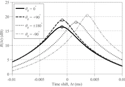
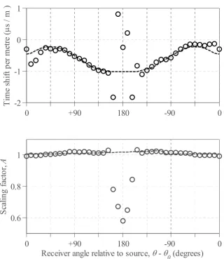
Figure 2.18: Reduction factor, R(Δt), for the cylinder array from Figure 2.11 measured for a number of angles of incidence; θ = θ0+144°; cross-correlation values shown for reference

(circles) ...58 Figure 2.19: Time shift per metre (top) and scaling factor (bottom), both estimated (o) and polynomial fit (▬ ▬) for the measurement of the cylinder array of Figure 2.11; θ0 = -90°...60

Figure 2.20: Modelled (▬) and measured scattered pressure polar response for the cylinder array of Figure 2.11 using the subtraction method with (×) and without (o) the scaling and sample shifts obtained from Figure 2.19 applied; θ = θ0+180°, θ0 = -90°; f = 750Hz (top),

f = 3850Hz (bottom) ...61 Figure 2.21: 1×7 array of slats arranged according to a Maximum Length Sequence (MLS) [1 1 1 0 0 1 0]; arrangement (left) and measurement sample constructed at full scale (right).63 Figure 2.22: Measured (o) and modelled (BEM ▬, thin panel BEM ▬ ▬ ▬ scattered pressure polar response for the 1×7 array of slats as per Figure 2.21; θ0 = 0°; frequencies as listed ...64

Figure 2.23: 10×10 channel percolation structure; arrangement (top) and measurement sample constructed at 1:3 scale (bottom)...66 Figure 2.24: Measured (o) and modelled (BEM ▬, thin panel BEM ▬ ▬ ▬) scattered pressure polar response for the 10×10 channel percolation structure as per Figure 2.23; θ0 = 0°;

frequencies as listed...67 Figure 2.25: Measured and modelled scattered pressure for the 10×10 channel percolation structure as per Figure 2.23; θ0 = 0°; measured (top), thin panel BEM (bottom)...68

Figure 2.26: 10×10 optimised cylinder measurement sample constructed at 1:4 scale ...69 Figure 2.27: 10×10 optimised cylinder array arrangement ...70 Figure 2.28: Measured (o) and modelled (▬) scattered pressure polar response for the 10×10 cylinder array as per Figure 2.27; θ0 = 0° (left) and θ0 = 30° (right); frequencies as listed ...71

(11)

x

Figure 3.2: Geometry defining the extent of the Geometric Shadow Zone (GSZ) and Specular Zone (SZ) for a flat plate of width, D...78 Figure 3.3: Diffusion coefficient for 3 periods of an MLS ([+1 +1 +1 -1 -1 +1 -1]) binary Schroeder diffuser evaluated over the BSZ, GVZ and full circle of receivers; D = 1.81m,

f0 = 500Hz, θ0 = 0°, r0 = 20m, r = 10m. ...81

Figure 3.4: Normalised scattered pressure polar pattern for the diffuser as per Figure 3.3;

f = 1998Hz (▬), f = 2377Hz (▬ ▬) ...81 Figure 3.5: Normalised scattered pressure (top) and total pressure (bottom) for a flat plate;

D = 0.4m, rc = 2m, r0 = 5m, θ0 = 0°; f = 500Hz (▬ ▬), 1.5kHz (▬ ▬), and 2.5kHz (▬); central

shaded region depicts the approximate geometric shadow zone according to Eq. 3.1...83 Figure 3.6: Normalised scattered pressure with receiver distance in the forward-scattered region for a flat plate; D = 0.4m, r0 = 20m, θ0 = 0°, f = 2.5kHz; geometric shadow zone

according to Eq. 3.1 (▬ ▬) and far-field boundary as per Eq. 2.4 (▬ ▬ ▬) ...84 Figure 3.7 Scattering from a single cylinder of width D = 1.6m for a number of receiver distances; polar plots with frequencies as listed (top), and diffusion coefficient evaluated over the GVZ (bottom); r0 = 200m, θ0 = 0°...85

(12)

List of Figures

xi

Figure 3.13: Diffusion coefficient for a single cylinder evaluated over the RSZ for a range of receiver distances; D = 1.6m, r0 = 200m, θ0 = 0°; infinite far-field case modelled according to

Eq. 2.23...95 Figure 3.14: Normalised scattered pressure with receiver distance in the forward-scattered region for the cylinder array as per Figure 2.27; D = 1.52m, r0 = 200m, θ0 = 0°, f = 400Hz

(bottom) and f = 3kHz (bottom); Fresnel zone boundaries according to Eq. 3.3 (horizontal dashed lines) and far-field boundary as per Eq. 2.4 (dot-dashed line) ...97 Figure 3.15: Diffusion coefficient for a cylinder array as per Figure 3.14 evaluated over the RSZ for a range of receiver distances...98 Figure 3.16: Diffusion coefficient for a percolation structure arranged as per Figure 2.23 evaluated over the RSZ for a range of receiver distances; D = 0.67m, θ0 = 0°, r0 = 40m...99

Figure 3.17: Back-scattered intensity ratio, LIR, as defined by Eq. 3.5, for the cylinder array of

Figure 2.27; D = 1.52m, r0 = 200m, θ0 = 0°...101

Figure 4.1: Cross-section of a BAD panel (left) and its volumetric slats equivalent (right); surface patches arranged according to the Maximum Length Sequence (MLS) [1 1 1 0 0 1 0]

...105 Figure 4.2: Binary Amplitude Diffuser (BAD) arranged according to a Maximum Length Sequence (MLS) [1 1 1 0 0 1 0], arrangement (left) and measurement sample constructed at full scale (right) ...107 Figure 4.3: Measured (o) and modelled (▬ ▬) normalised scattered pressure polar response for the BAD of Figure 4.2, including equivalent slats array modelled using the thin panel BEM (▬); θ0 = 0°; f = 2kHz (top) and f = 4kHz (bottom) ...108

Figure 4.4: Autocorrelation function (top) and power spectrum (bottom) for a unipolar MLS [1 1 1 0 0 1 0] (▬o▬) and equivalent bipolar MLS [1 1 1 -1 -1 1 -1] (▬ □ ▬)...110 Figure 4.5: Normalised scattered pressure polar response for a 1D array of slats comprising 3 periods of the sequence sn = [1 1 1 0 0 1 0]; thin panel BEM (▬) and Fourier approximation

(13)

xii

Figure 4.6: Diffusion coefficient for the slats array as per Figure 4.5; thin panel BEM (▬), Fourier approximation (▬ ▬), simplified Fourier approximation (▬ ▬ ▬), and reference plate of width, D = 2.1m (▀)...113 Figure 4.7: Approximation of the scattering from an array of slats comprising 3 periods of the sequence sn = [1 1 1 0 0 1 0]; sinc function (top), array considered as point scatterers (centre),

and their product (bottom)...115 Figure 4.8: Slats array arranged according to an N = 7 (perfect) Golomb ruler...117 Figure 4.9: Aperiodic autocorrelation function (top) and power spectrum (bottom) for a N = 7 Golomb ruler [1 1 0 0 1 0 1] (▬o▬) and MLS [1 1 0 1 0 0 1] (▬ □ ▬)...118 Figure 4.10: Diffusion coefficient for an array of slats arranged according to the N = 7 Golomb ruler [1 1 0 0 1 0 1] (▬), and MLS [1 1 0 1 0 0 1] (▬ ▬); θ0 = 0°, de = dy = 10cm; flat

plate of width, D = 0.7m (▀) shown for reference...119 Figure 4.11: Relationship between the AACF sidelobe energy and the diffusion coefficient of the DFT; all combinations of the unipolar N = 21, E = 12 sequence (×), and 3 periods of the MLS [1 1 1 0 0 1 0] (o)...121 Figure 4.12: AACF (top) and power spectrum (bottom) for the best N = 21, E = 12 sequence found from an exhaustive search (▬o▬) and 3 periods of the MLS [1 1 1 0 0 1 0] (▬ □ ▬) ...122 Figure 4.13: Diffusion coefficient (top) for an array of slats comprising 3 periods of the MLS [1 1 1 0 0 1 0] (▬), the optimal N = 21, E = 12 sequence (▬ ▬), N = 18, E = 7 minimum-redundancy array (▬ ▬ ▬), N = 18, E = 6 Golomb ruler (▬ ▬) and flat plate (▀) shown for reference; f = 250Hz normalised scattered pressure polar pattern shown for MLS and optimal arrangements only (bottom); θ0 = 0°, D = 2.1m...123

Figure 4.14: Normalised scattered pressure polar response for a 1D array of slats arranged according to an optimal N = 21, E = 12 sequence (▬), and an N = 18, E = 6 Golomb ruler (▬ ▬); f ≈ 1.8kHz, θ0 = 0°, D = 2.1m...125

(14)

List of Figures

xiii

Figure 4.16: Normalised scattered pressure polar response for an N = 7 Chebychev slat array; thin panel BEM (▬), and Fourier approximation (▬ ▬); f ≈ 1.2kHz (top) and f ≈ 2.4kHz (bottom); θ0 = 0°, D = 2.1m ...128

Figure 4.17: Diffusion coefficient for an N = 7 Chebychev slat array (▬), and an optimal

N = 21, E = 12 sequence (▬ ▬); θ0 = 0°; D = 2.1m; flat plate (▀) shown for reference ...129 Figure 4.18: Back-scattered intensity ratio for an array of slats arranged according to the

N = 21, E = 12 optimal sequence from Section 4.2.3 (▬), a flat plate of width D = 1.2m (▬ ▬), and a high frequency approximation as per Eq. 4.13 (▬ ▬ ▬); θ0 = 0°, D = 2.1m ...132

Figure 4.19: Back-scattered intensity ratio for a single slat of width de = 10cm (▬), the high

frequency approximation as per Eq. 4.13 (▬ ▬), and a line of best fit for the roll-on (▬ ▬ ▬); θ0 = 0°, D = 2.1m ...133

Figure 4.20: Back-scattered intensity ratio for an array of slats arranged according to the

N = 21, E = 12 optimal sequence from Section 4.2.3 (▬), approximate model – sum (▬ ▬), approximate model – individual runs of slats (▬ ▬ ▬); θ0 = 0°, D = 2.1m...136

Figure 4.21:Diffusion coefficient (top) and back-scattered intensity ratio (bottom) for an array of slats arranged according to an N = 12, E = 6 sequence (▬);θ0 = 0°; diffusion coefficient of

flat plate of width D = 0.912m (▀) shown for reference...139 Figure 4.22: A 2D slat array comprising M = 5 layers separated by distance, dx, each made up

of an N = 10 sequence of slats separated by slat width, de = dy...141

Figure 4.23: Example of a two layered slat array (slats only) and its Schroeder diffuser equivalent (slats and side walls / fins)...142 Figure 4.24: Back-scattered intensity ratio for an array of slats arranged according to the

N = 12, E = 6 sequence from Section 4.2.6 with orthogonal layer at a distance behind of

dx = 5cm (▬) and dx = 1m (▬ ▬); θ0 = 0°, D = 0.912m ...142

Figure 4.25: Illustration of the process for predicting the back-scattered intensity from a multi-layered array of slats with small layer spacing...144 Figure 4.26: Back-scattered intensity ratio for the dx = 5cm array as per Figure 4.24 (▬) and

(15)

xiv

Figure 4.27: Total pressure behind a single layered slat array comprising a single hole of width d = 22.8cm in the centre of a plate of width D (top) and the N = 12, E = 6 sequence from Section 4.2.6 (bottom); f = 6617Hz, θ0 = 0°...147

Figure 4.28: Geometry for determining the back-scattered intensity from a slat of width, d, situated at a distance, dx, behind a slit of the same width...148

Figure 4.29: Back-scattered intensity ratio for a slats array comprising alternating orthogonal layers based on the N = 12, E = 6 sequence from Section 4.2.6; M = 2 (▬), M = 5 (▬), and their respective approximate models (▬ ▬ ▬ and ▬ ▬ ▬); θ0 = 0°, dx = 1m, D = 0.912m ...150

Figure 4.30: Normalised scattered pressure for the two layered slat array as per Figure 4.23 (top) and equivalent Schroeder diffuser modelled using a Fourier approximation (bottom); θ0 = 0°, dx = 20cm, dy = de = 7.6cm ...153

Figure 4.31: Back-scattered diffusion coefficient for the two layered slat array as per Figure 4.23 (▬) and equivalent Schroeder diffuser modelled using a Fourier approximation (▬ ▬); θ0 = 0°, D = 0.912m, dx = 20cm, dy = de = 7.6cm; flat plate (▀) shown for reference ...154 Figure 4.32: Slat array arranged according to the locations of the well bottoms of an N = 7 Primitive Root Diffuser (PRD) (solid lines) and additional layers (dashed lines) ...155 Figure 4.33: Diffusion coefficient (back-scattered) for the slat arrays as per Figure 4.32; PRD slats only (▬) including additional layers (▬ ▬) and equivalent Schroeder diffuser modelled using a Fourier approximation (▬ ▬ ▬); θ0 = 0°, D = 1.8m, dx ≈ 7.2cm, dy = de = 30cm; flat plate

(▀) shown for reference ...156 Figure 4.34: Diffusion coefficient (back-scattered) as per Figure 4.33 though with angle of incidence, θ0 = +30°; flat plate (▀) shown for reference is for normal incidence ...157 Figure 4.35: Scattered pressure specular reflection off the slat array as per Figure 4.32 (PRD slats only); θ0 = 0° (▬), and +30° (▬ ▬); dx = 20cm ...158

Figure 4.36: M = 5 × N = 26 Golomb ruler slat array arrangement (a) and single layer equivalent as viewed by normal incidence source (b)...160 Figure 4.37: Diffusion coefficient for an M = 5 × N = 26 Golomb ruler array with layer spacing dx = 5cm (▬) and dx = 20cm (▬ ▬), and equivalent single layer array (▬ ▬); θ0 = 0°,

(16)

List of Figures

xv

Figure 4.38: Back-scattered intensity ratio for the slat array as per Figure 4.37...161 Figure 4.39: M = 5 layered Golomb ruler slat array arrangement based on an impedance matching approach (varying slat size with layer)...163 Figure 4.40: Diffusion coefficient (top) and back-scattered intensity ratio (bottom) for the slat array as per Figure 4.39; equal spacing (▬), Golomb ruler spacing (▬ ▬) and logarithmic layer spacing (▬ ▬ ▬); θ0 = 0°, D = 1.8m; flat plate (▀) shown for reference on top figure ..165 Figure 5.1: M×N Square grid bond percolation structure realised as a series of slats of width,

de; slats (▬), underlying grid (▬), and propagation paths (▬ ▬); circles denote nodes...173

Figure 5.2: Total pressure in a closed pipe of width d = 10cm with a 90° corner and totally absorbing termination at both ends due to a source (white circle) located at (-0.45, 0.45);

de/λ = 0.30 (top) and de/λ = 0.70 (bottom) ...175

Figure 5.3: Transmission round a 90° corner in a pipe as per Figure 5.2 ...176 Figure 5.4: N = 7 QRD (a) and reduced depth folded well equivalent (b) (after Cox and D’Antonio [3]); total depth dmax expressed as a fraction of the maximum well depth, d...177

Figure 5.5: Average (unwrapped) phase change on exit from the deepest well of 3 periods of the N = 7 QRD diffuser as per Figure 5.4; standard arrangement (▬), folded equivalent (▬ ▬) and simple phase change calculation using e2jkd (▬ ▬ ▬)...178 Figure 5.6: Baffled structures used to test the phase change on exit; de = 5cm, D = 10.0m,

θ0 = 0°; (dashed lines etc… indicate the propagation paths considered below) ...180

Figure 5.7: Phase change on exit from the structure of Figure 5.6 (a) (▬) compared to that predicted by ejkd for the short branch (▬ ▬), the long branch (▬ ▬), and the sum of the two (▬ ▬ ▬)

...181 Figure 5.8: Phase change on exit from the structure of Figure 5.6 (b) (▬) compared to that predicted by ejkd_{for the short (▬ ▬) and long (▬ ▬ ▬) routes to the dead end ...182}

(17)

xvi

Figure 5.10: Bond percolation surface diffuser (a) and the same structure lacking vertical (b) and horizontal (c) elements; Schroeder diffuser equivalent (d) ...184 Figure 5.11: Average diffusion coefficient for 1000 randomly generated 5×20 percolation bond surface diffusers with percentage of lattice lines filled: vertical (top), horizontal (middle) and total (bottom); de = 5cm, D = 1.0m, θ0 = 0°; grey circles indicate best 20 diffusers ...186

Figure 5.12: Diffusion coefficient for 1000 randomly generated 5×20 percolation bond surface diffusers with percentage of lattice lines in structure filled; vertical elements (top) and horizontal elements (bottom); de = 5cm, D = 1.0m, θ0 = 0°...188

Figure 5.13: Diffusion coefficient for 1000 randomly generated 5×20 percolation bond surface diffusers with percentage of line-of-sight filled; de = 5cm, D = 1.0m, θ0 = 0°...189

Figure 5.14: Average (solid lines) and maximum (dashed lines) diffusion coefficient obtained per frequency for 1000 randomly generated surface diffusers based on a 5×20 square grid lattice; bond percolation diffuser (▬)and equivalent Schroeder diffuser (▬); de = 5cm,

θ0 = 0°; reference plate of width D = 1.0m (▀) ...191 Figure 5.15: Best low frequency (a) and high frequency (b) diffusers from 1000 randomly generated percolation structures based on a 5×20 square grid lattice (top) and their diffusion coefficient (a ▬, b ▬ ▬) including plate of width D = 1.0m (▀) shown for reference (bottom); de = 5cm, θ0 = 0°...193

Figure 5.16: Diffusion coefficient for 1000 randomly generated 10×10 percolation bond volume diffusers with percentage of lattice lines filled: vertical (top) and horizontal (bottom);

de = 5cm, D = 0.5m, θ0 = 0°...195

Figure 5.17: Average diffusion coefficient for 1000 randomly generated 10×10 percolation bond volume diffusers with percentage line-of-sight blocked; de = 5cm, D = 0.5m, θ0 = 0°;

grey circles indicate best 20 diffusers...197 Figure 5.18: Example 10×10 percolation bond volume diffusers (top) and their corresponding ‘ant in a labyrinth’ results (bottom) including lines of best fit (dashed lines); de = 5cm,

D = 0.5m, θ0 = 0°...200

(18)

List of Figures

xvii

percolation bond volume diffusers; de = 5cm, D = 0.5m, θ0 = 0°; grey circles indicate best 20

diffusers ...201 Figure 5.20: Illustration of the Eden growth algorithm (progressing from left to right) starting with 3 seeds for the construction of a 4×4 tortuous square grid percolation structure...203 Figure 5.21: Best 10×10 percolation diffusers formed using the adapted Eden growth method grown from 1 (a), 10 (b) and 40 (c) seeds (top) and their diffusion coefficient (▬ (a), ▬ ▬ (b) and ▬ ▬ ▬ (c)) including reference plate of width D = 0.5m (▀) (bottom); de = 5cm, θ0 = 0°205

Figure 5.22: diffusion coefficient with range in effective well depth for 1000 randomly generated 10×10 percolation bond volume diffusers; , de = 5cm, D = 1.0m, θ0 = 0°...207

Figure 5.23: Average diffusion coefficient over the frequency range 313Hz ≤ f ≤ 4kHz with the standard deviation of the AACF sidelobes for 1000 randomly generated 10×10 percolation bond volume diffusers; de = 5cm, D = 1.0m, θ0 = 0°; grey circles indicate best 20 diffusers 208

Figure 5.24: Back-scattered intensity ratio including approximate power model from Chapter 4 (▬ ▬ ▬) (top) and diffusion coefficient including reference plate of width D = 1.0m (▀) (bottom) for the percolation bond surface diffusers from Figure 5.18 (a) (▬) and (c) (▬ ▬); de = 5cm, D = 0.5m, θ0 = 0°...210

Figure 5.25: Porous foam placed in the centre of the measured percolation structure from Section 2.6.2 (left) and its approximate location within the structure (hatched area, right);

de = 6.7cm (when scaled), θ0 = 0°...211

Figure 5.26: Average (normalised) back-scattered pressure from measurements for the percolation structure of Figure 5.25 without (▬) and with foam (▬ ▬)...212 Figure 5.27: Average normalised scattered pressure with frequency for 400 randomly generated percolation bond volume diffusers based on the grid types shown; de = 10cm,

D = 1.0m, θ0 = 0°...214

(19)

xviii

Figure 5.30: Examples of percolation volume diffusers based on a Bethe lattice (left) and a random node lattice with bonds determined by Delaunay triangulation (right); bonds are either occupied (▬) or vacant (▬ ▬ ▬) based on random selection...218 Figure 5.31: Average normalised scattered pressure with frequency for 400 randomly generated percolation bond volume diffusers based on a Bethe lattice; θ0 = 0°, D = 1.0m....220

Figure 5.32: Average normalised scattered pressure with frequency for 400 randomly generated percolation bond volume diffusers based on the random Delaunay triangulation construction method; θ0 = 0°, D = 1.0m ...221

Figure 5.33: Diffusion coefficient (top) and back-scattered intensity ratio (bottom) for the best random Delaunay triangulation (▬) and Bethe lattice (▬ ▬) percolation structures obtained via Monte Carlo simulation; θ0 = 0°; top plot includes plate of width D = 1.0m (▀) for reference ...223 Figure 5.34: Best diffuser obtained from the Monte Carlo simulation of 400 randomly generated percolation structures based on a z = 3 Bethe lattice (left) and a randomised Delaunay triangulation lattice (right) ...224 Figure 6.1: Normalised scattered pressure for a single cylinder of diameter, de, expressed

relative to wavelength...230 Figure 6.2: Normalised scattered pressure polar response for a 1D array of cylinders arranged according to an N = 7 Golomb ruler sequence sn = [1 1 0 0 1 0 1]; MS (▬) and Fourier

approximation (▬ ▬); θ0 = 0°, de = 10cm, dy = 20cm; frequencies as listed ...232

Figure 6.3: Diffusion coefficient for an array of cylinders of diameter de = 10cm arranged

according to the N = 7 Golomb ruler [1 1 0 0 1 0 1] (▬), and MLS [1 1 0 1 0 0 1] (▬ ▬); and an N = 7 Golomb ruler array of slats of width de = 20cm (▬ ▬); θ0 = 0°, dy = 20cm; flat plate of

width, D = 1.4m (▀) shown for reference ...234 Figure 6.4: Normalised scattered pressure polar response for an N = 7 Chebychev cylinder array; MS (▬), and Fourier approximation (▬ ▬); f = 1.5kHz (top) and f = 4.0kHz (bottom); θ0 = 0°, dy = 20cm, D = 1.4m...236

(20)

List of Figures

xix

Figure 6.6: Back-scattered intensity ratio for an array of cylinders arranged according to the

N = 7 Golomb ruler [1 1 0 0 1 0 1]; MS (▬), Fourier approximation (▬ ▬) and approximate model (▬ ▬ ▬); θ0 = 0°, dy = 20cm, de = 10cm, D = 1.4m ...239

Figure 6.7: Geometric reflection from an array of cylinders...240 Figure 6.8: Back-scattered intensity ratio for an array of cylinders as per Table 6.1 (a ▬, b ▬ ▬, and c ▬ ▬), and approximate model for array b (▬ ▬ ▬); θ0 = 0°, dy = 20cm, D = 1.4m ....242

Figure 6.9: Normalised scattered pressure with frequency; optimised arrangement as per Figure 2.27 modelled as point sources with spacing dx = dy = 16cm (a), single cylinder of

width de = 8cm (b), their product (c) and a full MS solution (d); θ0 = 0°...247

Figure 6.10: Diffusion coefficient for the optimised cylinder array as per Figure 2.27; MS (▬), Fourier approximation (▬ ▬) and predicted Bragg frequencies (· · ·); θ0 = 0°; flat

plate (▀) shown for reference...248 Figure 6.11: Fourier domain representation of the scattering from the arrangement as per Figure 2.27 (considered as point sources) for a number of wavelengths; d = dx = dy, θ0 = 0°249

Figure 6.12: Back-scattered intensity ratio for the optimised cylinder array as per Figure 2.27; MS (▬), Fourier approximation (▬ ▬), approximate model (▬ ▬ ▬) and predicted Bragg frequencies (· · ·); θ0 = 0°...252

Figure 6.13: Amplitude shaded Chebychev cylinder array arrangement (top) and polar pattern (bottom) for frequencies f = 750Hz (▬) and f = 1.5kHz (▬ ▬); θ0 = 0°...254

Figure 6.14: Diffusion coefficient for the amplitude shaded Chebychev array as per Figure 6.13; MS (▬), and predicted Bragg frequencies (· · ·); θ0 = 0°; flat plate (▀) shown for reference ...255 Figure 6.15: Construction of a Taylor T4 variant (N = 15) Costas array from a Lempel L2

(N = 17) construction...257 Figure 6.16: N = 15 Taylor T4 Costas arrangement of cylinders (top) and AACF (bottom)..258

Figure 6.17: Diffusion coefficient (top) and back-scattered intensity ratio (bottom) for the

(21)

xx

Figure 6.18: Scattered pressure for a 15×15 square grid array of point scatterers; θ0 = 0°,

d = dx = dy...261

Figure 6.19: Diffusion coefficient for the N = 15 Costas cylinder array as per Figure 6.16 with varying cylinder size de (relative to cylinder spacing d = dx = dy) ...261

Figure 6.20: Transformation of a 7×7 Lempel L2 Costas array from a square lattice to a

hexagonal lattice via shearing and then compression (shear-compression) – after Golomb and Taylor [78]...263 Figure 6.21: Square grid (a) and transformed hexagonal array (b) for a 27×27 Lempel L2

Costas construction, along with respective AACF vector spacings (c) and (d). ...264 Figure 6.22: Modelled diffusion coefficient (top) and back-scattered intensity ratio (bottom) for a hexagonal Lempel L2 Costas array of cylinders; equal sized cylinders, de = 10cm (▬)

and amplitude shaded array as per Figure 6.23 (▬ ▬); θ0 = 0°, D = 2.04m; diffusion coefficient

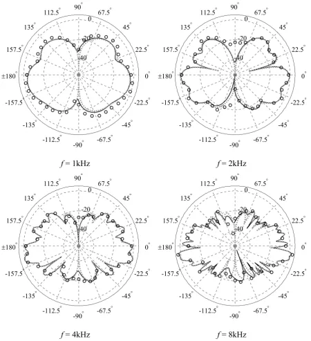
of flat plate (▀) shown for reference ...265 Figure 6.23: Hexagonal amplitude shaded cylinder measurement sample constructed at 1:4 scale ...267 Figure 6.24: Random incidence (back-scattered) diffusion coefficient for the amplitude shaded array as per Figure 6.23; modelled (▬) and measured (▬ ▬); D = 2.04m; diffusion coefficient of flat plate (▀) shown for reference...268 Figure 7.1: Volume diffusion coefficient (▬) and Back-scattered diffusion coefficient (▬ ▬) for the amplitude shaded cylinder array of Figure 6.22 modelled using the multiple scattering technique; θ0 = 0°, D = 2.04m; flat plate (▀) shown for reference...273 Figure 7.2: Bilsen’s (normalised) colouration metric (from prediction models) for the amplitude shaded cylinder array shown in Figure 6.23 (top) and 5 periods of a length 7 QRD Schroeder diffuser (bottom); D = 1.6m, θ0 = 0°...281

(22)

List of Figures

xxi

(23)

xxii LIST OF TABLES

(24)

Glossary of symbols and abbreviations

xxiii

GLOSSARY OF SYMBOLS AND ABBREVIATIONS

Symbols

a Cylinder radius

A Scaling term

Al,m Matrix of surface interactions

An , Am,n Set of amplitude coefficients

An′ Transmitted amplitude coefficients

Ani Set of coefficients for a multiple scattering solution

AS Effective absorption area according to Sabine’s equation

AT Transformation matrix

c Speed of sound (ms-1)

ca Ant in a labyrinth constant

c1, c2 Sound speeds during respective measurements (ms-1)

Ca(τ) One-dimensional Aperiodic Autocorrelation Function (AACF)

CA(τ,ρ) Two-dimensional Aperiodic Autocorrelation Function (AACF)

Cm,n Matrix defining a Costas array

d Distance (m)

de Element width (m)

dm Depth of the mth layer (m)

dmax Maximum layer depth (m)

dmin Minimum layer depth (m)

dn Width of the nth element (m)

drun Width of continuous run of conjoined elements (m)

dx Grid spacing in the x direction (m)

dy Grid spacing in the y direction (m)

dz Grid spacing in the z direction (m)

dτ Time constant (s)

D Diffuser width (m)

Dmax Maximum diffuser dimension (m)

e Scattered polar pattern for an individual scattering element

(25)

xxiv E Number of scattering elements

Error(f) Cancellation error – frequency domain

Errorref(f) Normalised cancellation error – frequency domain

f Frequency (Hz)

fc Cut-off frequency (Hz)

fmax Diffuser upper limiting frequency (Hz)

fs Sampling frequency (Hz)

f0 Diffuser design frequency (Hz)

Ffill Fraction of line-of-sight through an array that is blocked

ga Ant in a labyrinth gradient

G Green’s function

h1(t) Impulse response of measurement with sample present

h1'(t) Time shifted version of measurement with sample present

h2(t) Impulse response of background measurement (without sample present)

h3(t) Impulse response of loudspeaker and microphone

h4(t) Deconvolved sample Impulse response

Hn(1)(x) Hankel function of the first kind of order n

i Integer

Im Back-scattered intensity ratio from the first m layers

I Identity matrix

j _{Imaginary unit (} _₁₎

Jn(x) Bessel function of the first kind of order n

k Wavenumber (m-1)

k1, k2 Wavenumber during respective measurements (m-1)

l Integer

L Length of a Golomb ruler

Lr Length of surfaces within a room

LIR Back-scattered intensity ratio (dB)

Lp Sound pressure level (dB)

m Integer

M Number of modes

(26)

xxv

n Integer

n Normal to the surface (pointing out of the surface) N Number of rows in an array of scattering elements

N Number of elements

pb Bond probability

pbc Bond percolation threshold

pi Incident pressure (Pa)

pi,ref Incident pressure at the reference receiver (Pa)

ps Scattered pressure (Pa)

ps,norm Normalised scattered pressure

pt Total pressure (Pa)

p1,n , p2,n Scattered pressure at the nth receiver for respective cases (Pa)

P Number of elements per period Pi Matrix of incident pressures

Pt Matrix of surface pressures

q Prime number

r Receiver distance (m)

r Receiver location

ra, rb Arbitrary locations

ri Centre of the ith cylinder

rl Centre of the lth cylinder

rmax Maximum distance between source and diffuser surface (m)

rmin Minimum distance between source and diffuser surface (m)

rref Source to reference receiver distance (m)

rn Distance to the centre of the nth scattering element

rn Centre of the nth scattering element

rs Point on surface

r0 Source location

r0 Source distance (m)

R Set of receivers

R Pressure reflection coefficient

(27)

xxvi R(Δt) Reduction factor (dB)

s Surface

S Source

Sr Area of 2D room

S′ Image source

t Time (s)

TE Reverberation time predicted using Eyring’s equation(s)

TS Reverberation time predicted using Sabine’s equation(s)

u Primitive root

v Primitive root

x Cartesian coordinate (m)

x Variable

xt Transformed x Cartesian coordinate (m)

y Cartesian coordinate (m)

yt Transformed y Cartesian coordinate (m)

z Cartesian coordinate (m)

z Specific acoustic impedance (kgm-2s-1)

z Bethe lattice number

Zni Set of coefficients determined by boundary conditions

α Absorption coefficient

α Integer

 Mean absorption coefficient

β Surface admittance – inward facing normal (rayl-1)

β Integer

β' Surface admittance – outward facing normal (rayl-1)

δ Delta function

δ Diffusion coefficient

Δc Difference in speed of sound (ms-1) Δr Difference in distance (m)

Δt Time shift (s)

θ Angle of azimuth (radians)

(28)

xxvii

θl,i Angle between the ith and lth cylinder (radians)

θl,0 Angle between source and lth cylinder (radians)

θ0 Source angle (radians)

λ Wavelength (m)

ρ Autocorrelation lag (x dimension) ρ0 Density of air (kgm-3)

τ Autocorrelation lag (y dimension)

τ1, τ2 Time of flight for respective measurements (s)

φ Solid angle defining the shadow zone behind a diffuser (radians) φ Angle of elevation (radians)

φ0 Source angle of elevation (radians)

Ω External region (to the scattering objects) Ω Angular variable (radians)

Ω0 Internal region (of the scattering objects)

ψ Allowed angles of reflection

ψ(f Solid angle defining the interfering scattered zone behind a diffuser

n Neumann symbol

Abbreviations

AACF Aperiodic Autocorrelation Function

ACF Autocorrelation Function

ASSR Average Sidelobe to Specular Ratio BAD Binary Amplitude Diffuser

BEM Boundary Element Method

BSZ Back-Scattered Zone

DFT Discrete Fourier Transform

FT Fourier Transform

FSZ Forward-Scattered Zone

GSZ Geometric Shadow Zone

GVZ Geometric Visible Zone

(29)

xxviii

MS Multiple Scattering

PRD Primitive Root Diffuser QRD Quadratic Residue Diffuser

RT Reverberation Time

(30)

Acknowledgements

xxix ACKNOWLEDGEMENTS

It would not have been possible to have written this thesis without the help and support of many people. It is not possible to mention each and every one of them here, though I will endeavour to include those to which I am particularly grateful.

Above all I wish to express thanks to my partner Lucy for her patience, support and words of encouragement. I am also extremely grateful for the support of my immediate family, my parents Kathryn and Gareth and my sisters Laura and Alex; and to my closest friends. I also include in this Lucy’s parents Brian and Pam, who have shown great support to me throughout.

I would like to express my gratitude towards Professor Trevor Cox and Professor Jamie Angus for the help they provided throughout my studies. In particular, I would like to thank Professor Trevor Cox for his encouragement, guidance and dedication towards helping me complete this project; his knowledge and expertise providing a wealth of input.

I wish to acknowledge the input of the staff and my fellow postgraduates in the Acoustics Research Centre at the University of Salford for many helpful discussions and words of advice. There are too many to mention in person, though in particular I am grateful to Konstantinos Dadiotis for his help on the subject, notably through our many hours of discussions on diffusers which have proved invaluable to my research.

For there help with the construction of measurement samples I would like to express my thanks to Mike Clegg and Phil Latham of the University of Salford.

I would like to thank the Engineering and Physical Sciences Research Council (EPSRC) for funding the initial project on which the thesis is based (EP/D031745/1).

(31)

xxx DECLARATION

This is a declaration that the contents of this thesis are, except where due acknowledgement has been made, the work of the author alone. The following provides a list of publications associated with the research:

Publications

Hughes, R. J., Angus, J. A. S., Cox, T. J., and Umnova, O., "Volumetric Diffusers," Proc.

124th Convention Audio Eng. Soc., Amsterdam, The Netherlands, May 17-20, Convention

Paper No. 7432 (2008)

Hughes, R. J., Angus, J. A. S., Cox, T. J., Umnova, O., Whittaker, D. M., Gehring, G. A., and Pogson, M., "Volumetric Diffusion from Pseudorandom Periodic Cylinder Arrays," Presented

at the 8th European Conference on Noise Control (Euronoise), Edinburgh, Scotland, October

26-28 (2009)

Hughes, R. J., Angus, J. A. S., Cox, T. J., Umnova, O., Gehring, G. A., Pogson, M., and Whittaker, D. M., "Volumetric diffusers: Pseudorandom cylinder arrays on a periodic lattice,"

(32)

Abstract

xxxi ABSTRACT

Most conventional diffusers are used on room surfaces, and consequently can only operate on a hemispherical area. Placing a diffuser in the volume of a room may provide greater efficiency by allowing scattering into the whole space. There are very few examples of volume diffusers and they tend to be limited in design; subsequently a suitable method for their development is lacking.

2D volumetric diffusers are investigated, considering a number of design concepts; namely arrays of slats, percolation structures and cylinder arrays. An experimental technique is adapted for their measurement, and the results are used to verify prediction models for each type. Diffusive efficacy is assessed through a new metric based on an existing surface diffuser coefficient and a measure of scattered power requiring half of the energy to be back-scattered. Single layer slat arrays are formed from optimal aperiodic sequences, though due to the directional scattering from individual slats at higher frequencies, performance is heavily dependent on line-of-sight through the array. This limits the operational bandwidth to approximately 1.5 octaves. Multi-layer structures offer improvements by allowing cancellation of the back-scattered lobe, though at high frequency the specular reflection from an individual slat still dominates. Percolation fractals use slats orientated in multiple directions and by scattering laterally can channel sound and diffuse at lower frequencies. Low frequency diffusion however is limited and the best structures are those which provide a broad range of geometric reflection paths.

(33)

1 1. INTRODUCTION

1.1. Introduction

The design of a room, including surfaces and contents, can have a dramatic effect on the acoustic quality of the space. An acoustic environment determines the blend of direct and reflected sounds from sources, and ultimately how the sound in a space is perceived [1]. The use of diffusers as an acoustic treatment is well established, for example to reduce the effect of echoes. Problems such as strong echoes introduce distortion (unwanted artefacts caused by a listening environment) such as colouration (an uneven response with frequency); however it is often desirable to reduce such artefacts without removing energy from the room. Acoustic diffusers aim to both spatially and temporally distribute their scattered energy in an optimal manner over a desired bandwidth, and therefore reduce these unwanted effects without the need for absorption [2]. Diffusion has therefore become an important feature in the design of many acoustically sensitive locations, such as concert halls, studios and auditoria.

The research presented in this thesis investigates a new type of diffuser, one which operates in the volume of a space. This ‘volume diffuser’ is different to most conventional diffusers which generally take the form of a surface based treatment.

Although some volumetric diffusers do exist, the design process behind them has so far been limited, and installations tend to be application specific. Any device would ideally therefore take the form of a versatile ready-to-install stand alone unit, intended for a variety of room types and applications, which would add to the tools at the disposal of the acoustic engineer. To date however no one has designed, tested, or examined the potential application of such diffusers in any depth. Consequently there is a lack of an appropriate methodology for their design, measurement and analysis, and it is this that forms the basis of the work.

(34)

Chapter 1: Introduction

2

statement of the aims and objectives of the work are presented. Finally an outline of the thesis structure as a whole is given.

1.2. An introduction to architectural acoustics

In most environments the sound that we hear is a combination of the direct sound from a source or sources, and the indirect sound from reflections off the surfaces and objects within a space. This combination of direct and reflected sound determines how the space is perceived [1]. Architectural acoustics is concerned with this relationship in the built environment; for example in a large concert hall the walls, ceiling, floor and objects within the space will provide many reflections which determine the overall acoustic. By manipulating the reflections from these surfaces and/or objects, along with other important factors such as room volume and shape, the acoustic environment may be altered to best suit the intended use [3].

The design of architectural spaces as listening environments has a long and rich history. Examples stretch from the fan and elliptical arenas of ancient Greece and Rome, through to the classic theatres, opera houses and concert halls of the 18th and 19th Centuries [4]. The birth of modern architectural acoustics however is often cited as occurring a little over a century ago, with Sabine’s discovery of the relationship between the random incidence absorption coefficient and Reverberation Time (RT) [5]. This led to a considerable effort being devoted to the study of both surface absorption [3] and the required reverberation time of spaces such as auditoria [4; 6].

(35)

3

The work presented here investigates the design of diffusing structures. Many early (and perhaps accidental) examples of diffusers can be seen in the intricate decorative architectural features of classical halls; such as plaster mouldings, statuettes and coffered ceilings [4]. These irregularly shaped surfaces diffuse perhaps more by accident than design, though have later helped to inspire the installation of more purpose built structures, for example the ceiling of the Beethovenhalle in Bonn which comprises a series of arbitrarily arranged shapes such as hemispheres, pyramids and truncated cylinders [4]. Such structures provide diffusion due to their varying depth, absorbing properties, and scattering angles; however apart from very simple constructions they do not scatter sound in a predictable manner [9]. Sparked by the work of Schroeder [7; 8], modern diffusers which scatter in a more controlled manner are now widely used [3]. Relevant examples of these to the work presented here are introduced in Section 1.3.

1.3. Surface diffusers: important developments, concepts and limitations

(36)

[image:36.595.96.534.105.343.2]

4

Figure 1.1: Scattering from a 1D planar (left) and hemispherical (right) surface Schroeder

diffuser (after D’Antonio and Cox [2])

1.3.1 Schroeder diffusers

In his seminal paper of 1975 Manfred Schroeder posed the question:

“What wall shape has the highest possible sound diffusion, in the sense that an incident wave

from any direction is scattered evenly in all directions?” [7]

In this work Schroeder introduced the concept of a new type of diffuser to improve sound diffusion in concert halls and reverberation chambers; the phase grating diffuser. These diffusers were based on number theoretic pseudorandom sequences such as binary Maximum Length Sequences (MLS), which were later improved upon with integer based designs such as the Quadratic Residue Diffuser (QRD) [8] and the Primitive Root Diffuser (PRD) [10]. Often referred to as Schroeder diffusers, examples of which are depicted in Figure 1.1, these surfaces scatter sound in a controlled way.

A Schroeder diffuser comprises a series of equal width wells of varying depth, dn, separated

(37)

5

travelled (a concept particularly relevant to the slats and percolation diffusers presented in Chapters 4 and 5). This then results in dispersion due to interference between the reradiated waves. The well depths are usually determined by an appropriate number theoretic sequence,

sn, which when repeated periodically is designed to emphasise the energy scattered into the

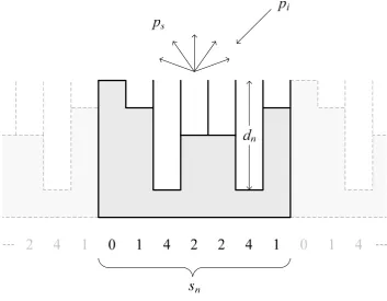
grating lobes. A QRD for example scatters equal energy into these lobe directions, resulting in what Schroeder described as ‘optimal’ diffusion’ [8]. Figure 1.2 shows a cross-section through an example of a Schroeder diffuser: a planar length 7 QRD, highlighting a single period where the well depths are proportional to the quadratic residue sequence

sn = [0 1 4 2 2 4 1]. Here pi is the pressure incident from a source and ps is the scattered

[image:37.595.134.488.313.588.2]

pressure.

Figure 1.2: Cross-section of a Schroeder (phase grating) diffuser highlighting one period of a

repeated sequence; depths dn determined according to the quadratic residue sequence

sn = [0 1 4 2 2 4 1]

Limitations

(38)

6

significant diffusion between multiples of the design frequency. Their bandwidth of operation however can be limited by a number of factors, and these are considered below.

Low frequency – Performance is inherently restricted by available depth, since sufficient phase change is required on reflection. The lower cut-off frequency is often quoted as being equal to the design frequency, since this is the first point at which even energy diffraction lobes are achieved. The period width (width of a single diffuser) however must be greater than a wavelength to ensure that there is more than one grating lobe in the polar response, thus taking advantage of their equal energy [3]. Dependent on sequence choice a low frequency limit generally equates to a wavelength on the order of approximately twice the maximum depth, though scattering behaviour usually differs from that of a plane rigid surface for an octave or two below this [11].

High frequency – The design theory assumes that plane wave propagation dominates within the wells. Consequently this breaks down when a half wavelength becomes equal to the well width, and cross-modes begin to occur in the wells. This does not stop dispersion, but is a limit to how the theory is applied and hence when diffusion is achieved in a controlled manner. In addition to this the use of integer based sequences results in critical frequencies, occurring when all of the well depths are integer multiples of half a wavelength and their phase change on exit is equal. These are often referred to as plate frequencies, since this causes the diffuser to behave like a plane surface and reflect in a specular manner.

1.3.2 Amplitude diffusers

(39)

7

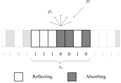
As with Schroeder diffusers, the use of number theoretic sequences allows the design of amplitude diffusers that scatter in a more controlled manner. These are referred to as amplitude grating diffusers [13], though due to both their absorbing and diffusing properties are also often referred to as hybrid diffusers. This concept was first used by Angus [13; 14] in the development of the Binary Amplitude Diffuser (BAD); so called as their surface arrangement is determined by a unipolar binary sequence, with values of 1 and 0 representing total reflection and total absorption respectively. An example of this is illustrated in Figure 1.3, where the MLS sn = [1 1 1 0 0 1 0] has been used. Like the Schroeder diffuser of Figure

1.2 the sequence is periodic, and hence sn represents a single period (highlighted).

Reflecting

Absorbing

p

i

p

s

1

0

1

0

1

0

1

[image:39.595.100.522.294.583.2]

s

n

Figure 1.3: Cross-section of an amplitude grating diffuser highlighting one period of a repeated sequence; surface patches arranged according to the Maximum Length Sequence

sn = [1 1 1 0 0 1 0]

Limitations

(40)

8

large auditoria where preservation of energy is required. One potential advantage is that unlike a welled diffuser there is (theoretically) no depth requirement (other than that required to fit the absorbent material). Since no phase change is introduced however, there is an inherent coherent specular reflection (though of a reduced amplitude relative to a rigid panel of the same size due to the use of absorption). Consequently sequences such as MLS often used in BAD panels are only able to scatter equal energy into the remaining (non-specular) grating lobes. Attempts have been made to reduce this effect, such as using curved surfaces [3], and more recently through a varying size patch design [15]. There are however several underlying limitations to performance:

Low frequency – Diffusive performance is limited by the properties of the absorbent material used. In practice the absorption must be on the order of a quarter wavelength deep to effectively remove energy, meaning that the theoretical lack of required depth does not hold true. Strictly speaking the slower sound speed of the absorption will mean that the depth requirement is reduced [3], though the need for depth is still an issue. Also, like the Schroeder diffuser, the period width must be greater than a wavelength to ensure the device works correctly when periodically repeated.

High frequency – Performance is limited by the directivity of the flat patches, since once wavelength is comparable to patch size an increasingly specular reflection results. Note this is also true for Schroeder diffusers, though their ability to alter the phase of a reflection means that this is less of a problem.

1.3.3 Other relevant surface diffusers

(41)

9

Geometric shapes such as triangles / pyramids can be used to perturb an incident wavefront by redirection and modulation [3]. Redirection may be of particular interest in the development of the volumetric diffuser for channelling of energy through a structure, in particular the percolations structures presented in Chapter 5.

1.4. A volume diffuser

1.4.1 Why a volume diffuser?

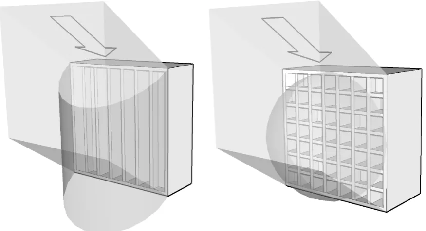
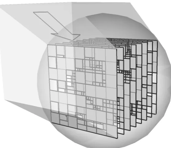
Most conventional acoustic diffusers take the form of a surface treatment, such as those discussed in Section 1.3 above. This means that they can only operate in 2π (hemispherical) space, with the remaining scattering paths being blocked off since these lie outside of the room. By considering a structure placed in the volume of the room, it becomes possible to operate on the full 4π (spherical) space, receiving from and scattering into all possible directions [3]. Such a structure forms a volume diffuser, an example of which is illustrated by Figure 1.4. This provides a potentially more efficient method of dispersing sound [3; 16], allowing a theoretical fourfold increase in efficiency relative to an equivalent sized surface diffuser. This occurs since the area received from and scattered into both double; a diffuser sees a twofold increase in both the rate at which it may interact with the sound incident upon it and the area over which it may spatially spread its reflections.

An important concept in the volume diffuser approach is that any device will likely be introduced into a location that was previously empty, thus introducing additional scattering surfaces. This is intrinsically different to the mechanism of a surface diffuser, which aims to alter the scattering characteristics of the surface it replaces. This was explained eloquently by Kuttruff in the statement:

“Quite a different method of achieving a diffuse sound field is not to provide for rough or corrugated walls, and thus to destroy specular reflections, but instead to disturb the free

(42)

[image:42.595.176.455.96.336.2]

10

Figure 1.4: Scattering from a 3D spherical volume diffuser

For example objects may be placed in the paths of strong echoes to scatter energy before an echo occurs; or in the paths of modal propagation, breaking up standing waves and creating a more uniform sound field both spatially and with frequency [3]. The latter is a solution adopted in many reverberation chambers, discussed in more detail in Section 1.4.3 below. If these elements were to interfere with the functionality of a room, for example being situated in the line-of-sight from an audience to a stage in an auditorium, then this solution would be impractical. Kuttruff [16] noted however that the method can be quite efficient even when only applied to parts of a room.

(43)

11

those seen in reverberation chambers; a construction which would likely be impractical for any surface diffuser.

Some surface diffusers rely on periodicity to produce their ‘optimum’ diffusion, which can be restricting as they only scatter evenly into the grating lobe angles, and periodicity is otherwise considered undesirable [3]. The use of periodicity has largely found favour due to reasons of practicality, since treating a surface is most easily achieved through a tiling based approach. Conversely a volume diffuser would be positioned in a spatial void, and consequently no longer needs to diffuse in conjunction with a series of neighbouring diffusers. This means that the restriction of periodic repetition of a base unit may be removed and the structure may form a diffusing object in its own right. Note this is not to say that a volume diffuser cannot be periodically repeated, though is a statement of their flexibility of placement.

1.4.2 Defining the volume diffuser

A volume diffuser may be defined as any object (or collection of objects) located in the volume of a space that alters the propagation of sound in a manner that promotes diffuse reflections and/or a diffuse field. The last part is important here, since to what extent a structure diffuses is a matter of definition. A surface diffuser for example promotes diffuse reflections to spread reflected energy both spatially and temporally, helping reduce unwanted artefacts that result from strong specular reflections. This is distinctly different to the approach adopted in many reverberation chambers, where a number of scattering surfaces hung within the space aim to create a diffuse field by redistributing energy, though do not necessarily promote diffuse reflections themselves.

To clarify the discrepancy above, in the context of the work presented here a more specific volume diffuser is referred to; one which forms a single stand alone unit that promotes diffuse reflections and acts as a diffuser in its own right. Ideally this would form a ready-to-install device suitable for application in a variety of room types. This definition is much more in keeping with that of a conventional surface diffuser, though with any need for repetition removed.

(44)

12

as the art installation shown in Figure 1.5, though these are analogous to the ornate surface decorations found in early auditoria which do not scatter in a controlled way. Conversely, whilst more purpose built structures (discussed in more detail in Section 1.4.3) scatter in a more predictable manner, they tend to be application specific and do not form a generic volume diffuser as defined above.

The design of a volume diffuser will essentially be limited only by size, which in turn is determined by available space. One constraint on these structures is that they cannot be placed where they interfere with a room’s functionality, for example in the line-of-sight of an audience. Examples such as absorbers being hung in large auditoria to control reverberation [3], or of chandeliers as mentioned above, suggest that dependent on the use of the space, it may be possible to find a number of suitable locations for volume diffusers. In reality additional factors such as practicality of construction, weight, and aesthetics will also be important, though these are not considered here.

(45)

13

1.4.3 Existing examples of acoustic volume diffusers

Reverberation chambers

Reverberation chambers often make use of suspended scattering surfaces hung within the room to promote a diffuse field by redistributing energy and breaking up modal propagation [3; 16], an example of which is shown in Figure 1.6. These may be viewed as a form of volume diffuser, for which current guidance on their application is given in Appendix A of international standard BS EN ISO 354:2003 “Acoustics – Measurement of sound absorption in a reverberation room” [18]. This recommends introducing a number of diffusing elements; specifically thin non-absorptive panels varying in size from 0.8-3m2 (for one side). These may be slightly curved and of random orientation and location. The actual number of diffusing panels to be used is essentially based on a trial and error process; a method which involves measuring the absorption coefficient of a test sample (assuming a diffuse field in accordance with Sabine’s equation [19]), and introducing diffusing panels until the average coefficient remains constant. In general the panels (considering both sides of each) should account for approximately 15-25% of the total surface area within the room.

(46)

14

Figure 1.6: Reverberation chamber with suspended scattering panels

(47)

15 Overhead stage canopies

Overhead stage canopies have been investigated for their effectiveness in controlling reflected sound to enhance intelligibility and clarity [20]. They are usually found suspended above a stage or audience in auditoria to reflect sound back into the space, for example back towards the musicians to allow them to hear what is being played and keep in time with one another [3]. A common criterion for their design is to achieve an even distribution of reflections over a defined area [21], and as such are similar in concept to surface diffusers. Since they are located in the volume of a space however, these may be viewed as a type of volume diffuser. Some canopies have virtually no open area and are curved to direct reflections sideways to promote lateral reflections and reduce colouration [8]. Of most interest to the work presented here however are canopy arrays, composed of a series of reflecting panels separated by intermediate gaps. By introducing these gaps the sound directed back to the stage may be controlled, whilst also permitting some sound to pass through the structure to be heard by the audience and to add to the general reverberance [3]. These arrays usually form a single layer of scattering panels, and as such are similar in concept to the 1D array volume diffusers presented later on in the thesis, in particular the 1D slat arrays presented in Section 4.2.

Rindel [22] determined that small elements were required in a canopy array so that diffracted energy was received in locations where there is no specular reflection, concluding that low frequency performance is determined by density and high frequency performance by panel size and spacing. Later Cox and D’Antonio [21] considered the effect of the density, size, shape and location of canopy elements using optimisation techniques, concluding that for high levels of support dense arrays of large simple shaped panels are best.