Optimizing deep learning networks using multi armed bandits

(1)

O

PTIMIZING

D

EEP

L

EARNING

N

ETWORKS

USING

M

ULTI

-A

RMED

B

ANDITS

Salem Abdussalam Ameen

School of Computing, Science and Engineering

College of Science and Technology

University of Salford, Manchester, UK

Submitted in Partial Fulfilment of the Requirements of the Degree of

Doctor of Philosophy

(2)

i

List of Tables

TABLE 2-1: EXAMPLE OF A SMALL DATA SET WHERE X0 AND X1 ARE FEATURES AND Y IS THE OUTPUT. ... 19

TABLE 3-1: SUMMARY OF RELATED WORK. ... 37 TABLE 4-1: A COMPARISON BETWEEN MULTI-ARMED BANDIT ALGORITHMS. ... 61

TABLE 5-1: CUMULATIVE AVERAGE REWARD FOR BOUNDED REWARDS WHEN PRUNING A

WEIGHT. ... 67

TABLE 5-2: CUMULATIVE AVERAGE REWARD FOR BINARY REWARDS WHEN PRUNING A

WEIGHT. ... 67

TABLE 5-3: WSLS UPDATED THE PROBABILITY P GIVING THE REWARD X AT EACH TRAIL. THE GREEN CELL REPRESENTS THE WEIGHT WITH THE HIGHEST PROBABILITY WHICH WILL BE

PLAYED AT THE NEXT. ... 72

TABLE 5-4: UCB1 METHOD WHERE X IS THE REWARD, N NUMBER OF PLAYS, T IS THE TOTAL

PLAYING TIME SO FAR, PF IS THE PADDING FUNCTION AND WJI IS THE WEIGHTS (THE

ALGORITHM WILL CHOOSE THE VALUE). ΜJI IS CUMULATIVE AVERAGE REWARD AND

GREEN COLOUR CELL IS THE ARM WILL BE PLAYED NEXT. ... 75

TABLE 5-5: RESULTS OF THOMPSON SAMPLING WHERE X IS THE CURRENT BINARY REWARD FOR EACH WEIGHT, T THE TOTAL PLAY TIME, S IS THE SUCCESS, AND F IS FAILURE AND

SAMPLE (BETA) IS DRAWN FROM THE BETA DISTRIBUTION FOR EACH WEIGHT. AT EACH TIME STEP, THE ALGORITHM WILL CHOOSE THE WEIGHT THAT HAS THE HIGHEST REWARD

AMONG THE OTHERS WHICH IS SHOWN IN THE GREEN CELL. ... 80

TABLE 5-6: RESULTS OF BAYESUCB ON DIFFERENT PLAY TIME WHERE X IS THE CURRENT

BINARY REWARD FOR EACH WEIGHT, T THE TOTAL PLAY TIME, S IS THE SUCCESS, AND F

IS FAILURE AND QUANTILE IS DRAWN FROM THE BETA DISTRIBUTION FOR EACH WEIGHT

WITH PROBABILITY 1-(1/T). AT EACH TIME STEP, THE ALGORITHM WILL CHOOSE THE

WEIGHT THAT HAS THE HIGHEST QUANTILE AMONG THE OTHERS WHICH IS SHOWN IN THE

GREEN CELL. ... 82

TABLE 5-7: UCI DATA SETS ... 85 TABLE 5-8: COMPUTED ERROR ON VALIDATION DATA SET BEFORE AND AFTER PRUNED THE

MODEL. THE GREEN CELL SHOWS THE METHOD WITH LESS ERROR WHILE RED CELL SHOWS

THE METHOD WITH LARGE ERROR. THE ARROWS POINT UP IF THE ERROR HIGH, DOWN IF IT

(6)

v

TABLE 5-9: RESULTS OF THE AVERAGE RANK OF THE METHODS ON 12 DIFFERENT DATA SETS. ... 88 TABLE 5-10: RUN-TIME PERFORMANCE IN SECONDS FOR THE DIFFERENT PRUNING METHODS

ON DIFFERENT DATA SETS. GREEN CELL SHOWS THE METHODS THAT HAVE LESS

COMPUTATION TIME WHILE THE RED CELL SHOWS THE ONES WITH THE HIGHEST

COMPUTATION TIME. ... 90

TABLE 5-11: NO OF PARAMETERS IN THE LENET’S MODEL... 91 TABLE 5-12: RESULTS OF PRUNING 50% OF TWO LAYERS IN THE LENET’S MODEL. ... 92 TABLE 6-1: CUMULATIVE AVERAGE REWARD FOR THE BOUNDED REWARDS WHEN PRUNING A

NEURON ON EXAMPLE OF DATA AT EACH FORWARD PROPAGATION. ... 97

TABLE 6-2: SOFTMAX FUNCTION FOR PRUNING THE NEURONS WHERE 𝜇𝜇𝜇𝜇 IS CUMULATIVE

AVERAGE REWARD, X IS GIVEN REWARD, 𝜏𝜏= 2 AND P IS THE PROBABILITY. ... 98

TABLE 6-3: THE STEPS OF CHOOSING NEXT NEURON TO PRUNE BASED OF HEDGE ALGORITHM. THE GREEN CELL IS THE PROBABILITY OF CHOOSING THE FOLLOWING NEURON. ρ IS THE GENERATED NON-STATIONARY REWARD, W IS THE WEIGHT AND P IS THE PROBABILITY

FOR CHOOSING THE NEXT NEURON. ϵ= 0.05. ... 99 TABLE 6-4: EXP3 FOR PRUNING THE NEURONS WHERE ρ IS THE CURRENT NON-STATIONARY

REWARD, W IS THE WEIGHT AND P IS THE PROBABILITY FOR CHOOSING THE NEXT NEURON

TO PLAY. Γ=0.1. GREEN CELLS ARE THE NEURONS CHOSEN TO PRUNE. ... 100

TABLE 6-5: SMALL DATA SET SPECIFICATION. ... 102 TABLE 6-6: DATA SET SPECIFICATION FOR DEEP LEARNING MODELS. ... 103 TABLE 6-7: HYPERPARAMETERS OF NEURAL NETWORKS TRAINED ON DIFFERENT DATA SETS.

IN ADDITION, THE LEARNING RATE FOR ALL OF THEM IS SET TO 0.001, THE ACTIVATION FUNCTION IS RELU AND THE NUMBER OF EPOCHS IS 100. ... 103

TABLE 6-8: COMPARISON OF ACCURACY BETWEEN PRUNING BASED ON UCB1 AND DIFFERENT CLASSIFIERS. THE RESULTS WITH RESPECT TO SOME CLASSIFIERS ARE NOT AVAILABLE IN

THE CASE OF THE FACE DATA SET BECAUSE OF THE RESOURCE REQUIRED. THE GREEN

CELLS INDICATE THAT THE METHOD HAS GOOD ACCURACY IN CONTRAST OF RED CELL.

THE ARROWS POINT UP IF THE ERROR HIGH, DOWN IF IT IS LOW OR IN RIGHT DIRECTION IF IT IS IN BETWEEN. ... 107

(7)

vi

DIFFERENT DATA SETS. IN THIS TABLE, THE HIGHEST IS THE BETTER AND THE TABLE IS

SORTED ON THE ACCURACY COLUMN. ... 108

TABLE 6-10: THE RESULT BASED ON THE ACCURACY OF PRUNING DEEP NEURAL NETWORKS ON

DIFFERENT DATA SETS USING DIFFERENT ARCHITECTURES. THE TABLE SHOWS THE

PRUNED LAYER, NUMBER OF NEURONS IN PRUNED LAYER AND THE PERCENTAGES OF

REMOVED NEURONS IN THE LAYER. THE GREEN CELLS INDICATE THAT THE METHOD HAS

GOOD ACCURACY IN CONTRAST OF RED CELL. THE ARROWS POINT UP IF THE ERROR HIGH,

DOWN IF IT IS LOW OR IN RIGHT DIRECTION IF IT IS IN BETWEEN. ... 115

TABLE 6-11: RESULTS OF RANKED ACCURACY RESULTS BASED ON NEMENYI TEST, WHICH IS USED TO COMPARE THE DIFFERENT MODELS ON SIX DIFFERENT DATA SETS. ... 124

TABLE 7-1: EXAMPLES OF COMPUTING FLOPS. ... 129 TABLE 7-2: RESULT OF PRUNING CONVOLUTIONAL LAYERS. THE GREEN CELLS INDICATE THAT

THE METHOD HAS GOOD ACCURACY IN CONTRAST OF RED CELL. THE ARROWS POINT UP IF

THE ERROR HIGH, DOWN IF IT IS LOW OR IN RIGHT DIRECTION IF IT IS IN BETWEEN... 136

TABLE 7-3: AVERAGE RANK OF THE ALGORITHMS FOR PRUNING FEATURE MAPS BASED ON ACCURACY, WHERE A HIGHER RANK IS BETTER. ... 137

TABLE 8-1: PRUNING USING MP-TS AND MP-UCB1. THE GREEN CELLS INDICATE THAT THE METHOD HAS GOOD ACCURACY IN CONTRAST OF RED CELL. THE ARROWS POINT UP IF THE

ERROR HIGH, DOWN IF IT IS LOW OR IN RIGHT DIRECTION IF IT IS IN BETWEEN... 147

TABLE 8-2: SUMMARY OF RESULTS BASED ON ACCURACY FROM THREE COMMON DATA SETS THAT WERE USED IN PRUNING BASED ON SINGLE OR MULTIPLE NEURONS OR FEATURE

MAPS. CELLS SHADED BLACK INDICATE THERE IS NO RESULT. CELLS SHADED GREEN HAS

BEST ACCURACY WHILE RED HAS THE WORSE. ... 148

(8)

vii

List of Figures

FIGURE 1.1: OVERVIEW OF THE THESIS STRUCTURE... 9

FIGURE 2.1: SGD FLUCTUATION . ... 15

FIGURE 2.2: THE EFFECT OF ADDING MOMENTUM TO GD. ... 16

FIGURE 2.3: EXAMPLE OF GRAPH OF MULTIPLE NODES. ... 20

FIGURE 2.4: DEFINITION OF A SINGLE NEURON WITH INPUTS, ACTIVATION FUNCTION AND OUTPUTS. ... 24

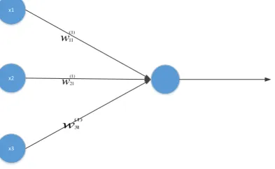
FIGURE 2.5: ARTIFICIAL NEURAL NETWORK WITH ONE HIDDEN LAYER WHERE W IS THE WEIGHT, B IS THE BIAS AND F IS A NON-LINEAR FUNCTION. ... 25

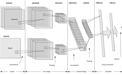
FIGURE 2.6: CONVNET MODEL WITH TWO INPUTS (INTENSITY AND DEPTH). ... 26

FIGURE 2.7: LENET MODEL [83]. ... 29

FIGURE 2.8: ALEXNET MODEL [22]... 29

FIGURE 2.9: RNN ARCHITECTURE. ... 30

FIGURE 2.10: LSTM ARCHITECTURE [100]. ... 31

FIGURE 2.11: END-TO-END MEMORY NETWORKS. (A): A SINGLE LAYER. (B): A MULTIPLE LAYER. ... 32

FIGURE 2.12: NEURAL NETWORKS (A) AFTER DROPOUT (B) AFTER DROPCONNECTION. ... 34

FIGURE 3.1: A TIMELINE OF RELATED ALGORITHMS. ... 37

FIGURE 5.1: BLOCK DIAGRAM SHOWS THE MAB TO PRUNE THE WEIGHTS. ... 64

FIGURE 5.2: THE GENERIC ALGORITHM OF A MAB PRUNING THE WEIGHS. ... 65

FIGURE 5.3: SYNTHETIC DATA FOR PURPOSE OF EXPLAINING MAB PRUNING ALGORITHMS. 66 FIGURE 5.4: FUNCTION OF EPSILON-GREEDY ALGORITHM TO PRUNE K WEIGHTS. ... 68

FIGURE 5.5: EPSILON-GREEDY FOR PRUNING 16 WEIGHTS AT DIFFERENT PLAY TIMES. THE RED DOTS DENOTE THE CHOSEN WEIGHT TO PLAYING. THE TOP ONE PLAYED FIRST AND THE BOTTOM ONE PLAYED THE LAST. ... 70

FIGURE 5.6: FUNCTION OF WSLS BASED ON PURSUIT ALGORITHM TO PRUNE K WEIGHTS. ... 71

FIGURE 5.7: FUNCTION OF UCB1 ALGORITHM TO PRUNE K WEIGHTS... 72

FIGURE 5.8: UCB1 FOR PRUNING 16 WEIGHTS AT DIFFERENT PLAY TIMES. STARTING FROM THE UPPER LEFT TILL THE BOTTOM AT DIFFERENT TIME. THE VERTICAL LINES REPRESENT THE CUMULATIVE AVERAGE REWARD (BOTTOM) AND THE PADDING FUNCTION (TOP). THE RED LINE IS CHOSEN FOR PLAYING. ... 74

(9)

viii

FIGURE 5.10: COMPUTE Q OF THE WEIGHT WHERE THE CHARTS ON THE TOP REPRESENT THE

WEIGHTS AT THE PLAY TIME BETWEEN (T=49 TO T=64). THEN, THE CHARTS AT THE

BOTTOM REPRESENT COMPUTING THE MAXIMUM Q FOR THE CURRENT CHOSEN WEIGHT.

... 77

FIGURE 5.11: THOMPSON SAMPLING WHERE THERE ARE K WEIGHTS AND 𝑤𝑤𝜇𝜇𝑤𝑤 IS THE WEIGHT SELECTED TO PLAY NEXT. ... 78

FIGURE 5.12: FUNCTION OF BAYESUCB TO PRUNE K WEIGHTS. ... 79

FIGURE 5.13: THOMPSON SAMPLING FOR CHOOSING THE ARM TO PLAY NEXT BASED ON THE SAMPLE FROM BETA DISTRIBUTION. THE TWO ARMS ON THE TOP ARE CHOSEN FROM THE FIRST COLUMN IN THE PREVIOUS TABLE WHILE THE CHARTS IN THE BOTTOM ARE CHOSEN FROM THE LAST COLUMN OF THE SAME TABLE. ON THE TOP, THE ALGORITHM WILL CHOOSE THE ARM ON THE LEFT AS IT HAS HIGHER REWARD WHILE ON THE BOTTOM THE ALGORITHM WILL CHOOSE THE ARM ON THE RIGHT AS IT HAS HIGHER REWARD. ... 81

FIGURE 5.14: BAYESUCB FOR CHOOSING THE ARM TO PLAY NEXT BASED ON THE SAMPLE FROM THE BETA DISTRIBUTION. THE TWO ARMS ON THE TOP ARE CHOSEN FROM THE FIRST COLUMN IN TABLE 5-5 WHILE THE CHARTS AT THE BOTTOM ARE CHOSEN FROM THE LAST COLUMN OF THE SAME TABLE. ON THE TOP, THE ALGORITHM WILL CHOOSE THE ARM ON THE LEFT AS IT HAS HIGHER QUINTILE WHILE ON THE BOTTOM THE ALGORITHM WILL CHOOSE THE ARM ON THE RIGHT AS IT HAS HIGHER QUINTILE ... 83

FIGURE 5.15: COMPARISON OF ALL CLASSIFIERS AGAINST EACH OTHER WITH THE NEMENYI TEST. LINES SHOW THE CRITICAL DIFFERENCE FOR EACH METHOD ANY GROUPS OF CLASSIFIERS THAT ARE NOT SIGNIFICANTLY DIFFERENT (AT P = 0.05) ARE OUT OF THE LINES. THE BLUE DOT SHOWS THE RANK MEAN WHILE THE LINE DETERMINE THE CD WHICH 4.33. ... 89

FIGURE 6.1: THE GENERIC ALGORITHM OF A MAB PRUNING NEURONS. ... 96

FIGURE 6.2: FUNCTION OF SOFTMAX ALGORITHM TO PRUNE K NEURONS. ... 98

FIGURE 6.3: THE HEDGE FUNCTION FOR PRUNING K NEURONS. ... 99

FIGURE 6.4: EXP3 FUNCTION TO PRUNE K NEURONS. ... 100

FIGURE 6.5: RESULTS OF MAB PRUNING ALGORITHMS. ... 106 FIGURE 6.6: COMPARISON OF THE ACCURACY OF ALL CLASSIFIERS AGAINST EACH OTHER WITH

THE NEMENYI TEST. HORIZONTAL LINES SHOW THE CRITICAL DIFFERENCE AWAY FROM

(10)

ix

ARE NOT SIGNIFICANTLY DIFFERENT (P = 0.0.5) ARE OUT OF THE LINES FROM PROPOSED

METHODS. CD=8.066. ... 110

FIGURE 6.7: COMPARISON OF THE F1 SCORE OF ALL CLASSIFIERS AGAINST EACH OTHER WITH THE NEMENYI TEST. HORIZONTAL LINES SHOW THE CRITICAL DIFFERENCE AWAY FROM

PROPOSED PRUNING METHODS AND ANY OTHER METHODS. GROUPS OF CLASSIFIERS THAT

METHODS ... 111

FIGURE 6.8: COMPARISON OF THE PRECISION OF ALL CLASSIFIERS AGAINST EACH OTHER WITH THE NEMENYI TEST. HORIZONTAL LINES SHOW THE CRITICAL DIFFERENCE AWAY FROM

METHODS. ... 112

FIGURE 6.9: COMPARISON OF THE RECALL OF ALL CLASSIFIERS AGAINST EACH OTHER WITH THE NEMENYI TEST. HORIZONTAL LINES SHOW THE CRITICAL DIFFERENCE AWAY FROM

METHODS. ... 113

FIGURE 6.10: COMPARISON OF ALL PRUNING ALGORITHMS AGAINST EACH OTHER WITH THE

NEMENYI TEST. HORIZONTAL LINES SHOW THE CRITICAL DIFFERENCE AWAY FROM

PROPOSED PRUNING ALGORITHMS, THE ORGINAL UNPRUNED MODEL AND TWO OTHER

ALGORITHMS THAT ARE NOT SIGNIFICANTLY DIFFERENT (P = 0.0.5) ARE OUT OF THE LINES

FROM PROPOSED ALGORITHMS. CD=3.218. ... 125

FIGURE 7.1 REMOVING THE FILTER ℱI,J AND CORRESPONDING FEATURE MAP IN XI+ 1 IN CONVNETS. THE TOP DIAGRAM SHOWS THE TWO LAYERS BEFORE PRUNING WHILE THE BOTTOM DIAGRAM SHOWS THE TWO LAYERS AFTER PRUNING THE FILTER AND FEATURE

MAP. ... 128

FIGURE 7.2: CHANGE IN TRAINING LOSS AS A FUNCTION OF THE REMOVAL OF A SINGLE FEATURE MAP FROM THE LENET MODEL. THE FIRST CONVOLUTIONAL LAYER IS ON THE

LEFT AND THE SECOND CONVOLUTIONAL LAYER IS ON THE RIGHT. THE TOP ROW SHOWS

THE RESULTS FOR BRUTE FORCE PRUNING, THE MIDDLE IS FOR UCB1 PRUNING AND THE

BOTTOM IS FOR THOMPSON SAMPLING. ... 132

(11)

x

FIGURE 7.4: COMPARISON OF ALL CLASSIFIERS AGAINST EACH OTHER WITH THE NEMENYI

TEST. HORIZONTAL LINES SHOW THE CRITICAL DIFFERENCE AWAY FROM PROPOSED

PRUNING ALGORITHMS AND ANY ALGORITHMS. CD=1.133. ... 138

FIGURE 8.1: PRUNING ALGORITHM BASED ON MP-MAB. ... 143

FIGURE 8.2: MP-TS FUNCTION WHERE THERE ARE K NEURONS OR FEATURE MAPS. ... 144

FIGURE 8.3: MP-UCB1 FUNCTION WHERE THERE ARE K NEURONS OR FEATURE MAPS. ... 144

FIGURE 8.4: PRUNING MULTIPLE NEURONS AT ONE TIME. ... 146

FIGURE 11.1: VISUALIZATION OF ABALONE DATA. ... 186

FIGURE 11.2: IMPORTANT FEATURES: ON THE TOP WINE QUALITY DATA SET AND ON THE BOTTOM GLASS DATA SET. ... 187

FIGURE 11.3: THE CORRELATION BETWEEN VARIABLES FROM LEFT TO RIGHT, PEARSON CORRELATION, SPEARMAN CORRELATION KENDALL CORRELATION. ... 189

FIGURE 11.4: PCA ON FACE DATA SET. THE 12 PHOTOS ON THE LEFT SHOW SAMPLES FROM THE DATA WHILE THE 12 ON THE RIGHT SHOW IMAGES AFTER APPLYING PCA. ... 191

FIGURE 11.5: HYPERPARAMETERS OF THE DECISION TREE ON BOSTON HOUSE DATA SET. .. 192

FIGURE 11.6: FINDING BEST COMBINATION OF PARAMETERS FOR ADABOOST. ... 194

FIGURE 11.7: ADABOOST ON BOSTON HOUSE DATA SET. ... 195

FIGURE 11.8: ROC ON ADULT DATA SET. ... 197

FIGURE 11.9: SOME CONFUSION MATRICES FOR THE PIMA DATA SET ... 198

FIGURE 11.10: R-SQUARED ON DIFFERENT MAB PRUNED MODELS ON X-AXIS SHOWS THE NUMBER OF PRUNED NEURONS AND IN Y-AXIS SHOWS THE ACCURACY. ... 215

FIGURE 11.11: R-SQUARED OF MAB ALGORITHMS AND THE ORIGINAL UNPRUNED MODEL TESTED ON REGRESSION TESTING DATA SETS ... 216

FIGURE 11.12: R-SQUARED BETWEEN MAB PRUNING ALGORITHMS PRUNED 25% OF THE ORIGINAL MODEL AND OTHER REGRESSION MODELS ... 218

(12)

xi

Dedication

This PhD Thesis is dedicated to all members of my family: My parents, who live abroad and kept their hearts with me.

My wife, Asia Ammar, for her support and patience with me throughout my PhD.

(13)

xii

Never give up. Today is hard, tomorrow will be worse, but the day after tomorrow will be

sunshine.

(14)

xiii

Acknowledgements

First, I would like to express my sincere gratitude to my advisor, Professor Sunil Vadera, for the continuous support in my PhD study and related research, for his patience, motivation, and immense knowledge. His guidance helped me in the research and writing of this thesis and, I could not have imagined having a better advisor and mentor for my study.

Besides my advisor, I would like to thank Professor Tim Ritchings for his time and encouraging words.

(15)

xiv

Declaration

This dissertation is the result of my own work and includes nothing, which is the outcome of work done in collaboration except where specifically indicated in the text. It has not been previously submitted, in part or whole, to any university of institution for any degree, diploma, or other qualification.

Signed: ______________________________________________________________

Date: _________________________________________________________________

(16)

xv

List of Abbreviations and Acronyms

The following table describes the significance of various abbreviations and acronyms used throughout the thesis.

Abbreviation Meaning

MAB Multi-Armed Bandit

ConvNets Convolution Neural Networks

RNN Recurrent Neural Network

LSTM Long Short-Term Memory

OBD Optimal Brain Damage

OBS Optimal Brain Surgeon

WSLS Win–Stay, Lose–Shift

UCB Upper Confidence Bound

KL-UCB Kullback-Leibler Upper Confidence Bound

BayesUCB Bayesian Upper Confidence Bound

EXP3 Exponential weight algorithm for Exploration and Exploitation

MP-TS Multi play Thompson Sampling

MP-UCB1 Multi play UCB1

TS Thompson Sampling

NN Neural Networks

E Greedy Epsilon Greedy

SM Softmax

(17)

xvi

Abstract

Deep learning has gained significant attention recently following their successful use for applications such as computer vision, speech recognition, and natural language processing. These deep learning models are based on very large neural networks, which can require a significant amount of memory and hence limit the range of applications.

Hence, this study explores methods for pruning deep learning models as a way of reducing their size, and computational time, but without sacrificing their accuracy.

A literature review was carried out, revealing existing approaches for pruning, their strengths, and weaknesses. A key issue emerging from this review is that there is a trade-off between removing a weight or neuron and the potential reduction in accuracy. Thus, this study develops new algorithms for pruning that utilize a framework, known as a multi-armed bandit, which has been successfully applied in applications where there is a need to learn which option to select given the outcome of trials. There are several different multi-arm bandit methods, and these have been used to develop new algorithms including those based on the following types of multi-arm bandits: (i) Epsilon-Greedy (ii) Upper Confidence Bounds (UCB) (iii) Thompson Sampling and (iv) Exponential Weight Algorithm for Exploration and Exploitation (EXP3).

(18)

Chapter 1: Introduction 1

Back propagation neural networks have a long history, dating back to the 1980s [1]. These neural networks consist of a network of connected neurons typically organized in layers. Layers are made up of many interconnected neurons which have a nonlinearity function known as an activation. Patterns or examples are presented to the network via the first layer which is known as the input layer, which communicates to one or more middle layer(s) known as the hidden layers where the actual processing is done via a system of weighted connections. The hidden layers then link to the last layer known as an output layer. The decades since their first development has seen many applications [2] of neural networks including in finance [3], a complete check reading system [4], in medical diagnosis [5-8], and in engineering[9-11]. More recently, there has been significant interest in using deep neural networks [12-18]. These deep neural networks consist of a sequence of feature recognition maps, building one layer on top the previous layer and where each layer aims to provide an abstraction of the previous layer, with the final layer performing classification [19]. For example, to recognize objects in images, the first layer aims to learn to recognize edges, the second layer combines edges to form motifs, the third learns to combine motifs into parts, and the final layer learns to recognize objects from the parts identified in the previous layer [20].

1. Introduction

(19)

Interest in these deep networks grew as a result of their success in the ImageNet Large Scale Visual Recognition Competition (ILSVRC)1 [21]. In 2012, Krizhevsky et al. [22] demonstrated significant performance improvements over the state of the art in the ImageNet benchmark challenge [21] with their deep network system AlexNet [22]. This has been followed by further advances with deep neural networks such as VGGNet [23], GoogLeNet [24], ResNet [25] and DenseNet [26].

These deep learning networks can become very large; for example, AlexNet has 8 layers and ResNet has 152 layers. Hence this thesis focuses on pruning their size. There are four aspects that motivate the need to prune deep neural networks:

• The first aspect is based on the view that neural networks should aim to mimic the brain to solve problems where each neuron relates to many others. If one accepts this view, which is expressed in most texts on the subject (E.g., Gurney [27]), then it is worth noting how the brain is believed to develop. The number of synapses are very large immediately after the human birth and this number increases sharply after a year from birth. Then, this number is pruned and stabilizes to 500 Trillion at the age of ten [28]. Hence if deep learning is to follow similar steps, they should adopt a pruning step to remove redundant and unimportant weights after developing the large networks [29].

• The second aspect involves using deep neural networks in embedded systems [30]. Currently, most applications of deep learning, such as image detection, natural language processing and speech recognition run on the cloud [31-33]. Running deep neural networks on mobile platforms is difficult at present given the size of the models [31-33].

• The third aspect is that reducing the size of models can speed up the prediction process [34]. This will be especially important for real time applications that use deep learning models [34, 35].

• The fourth aspect to note is that increasing the number of parameters (weights, biases, and neurons) does not necessarily grow the robustness or richness of the learned approximation, but might increase overfitting the data [36].

(20)

The primary solution pursued to address the above issues is based on Occam’s razor [37]: “Assume that an occurrence may have two explanations. Out of these, the simpler would generally be the better one”.

The problem addressed in this thesis is how best to do this in a way that reduces the size of the network but does not sacrifice performance.

Research on neural networks dates to the middle of the 20th century[38] while back propagation neural networks dates to the 1980s [1], and has thrived for many years, so not surprisingly, several techniques have already been developed for pruning neural networks; however, these techniques can be inefficient and very time consuming [39]. In this thesis, the goal is to study and develop algorithms for pruning deep neural networks more efficiently, leading to the following broad questions that need to be addressed:

1. How well do existing algorithms for pruning neural networks perform?

2. Can multi-armed bandit (MAB) best algorithms be developed for pruning and which methods work best?

3. How does the performance of the MAB based pruning methods compare with other methods?

Having identified the broad questions, the initial phases of research involved surveying the literature on deep learning, understanding existing methods and gaining practical experience with some applications. Practical experience was gained by using various development tools, such as the Torch scientific computing framework [40] to develop a deep network for American Sign Language. This initial work developed a convolutional neural network (ConvNets) aimed at classifying fingerspelling images using both image intensity and depth data. The developed convolutional network was evaluated by applying it to the problem of finger spelling recognition for American Sign Language. This initial work, in itself, produced better results than other published work and led to a journal publication [17]. It also led to a good understanding of deep learning architectures and a key observation that:

1.2. Research Problem

(21)

pruning deep neural networks involves a trade-off between accuracy and the number of the parameters pruned. That is, as we prune more and more neurons, feature maps or weights, the accuracy may reduce to a point where the network is not useful.

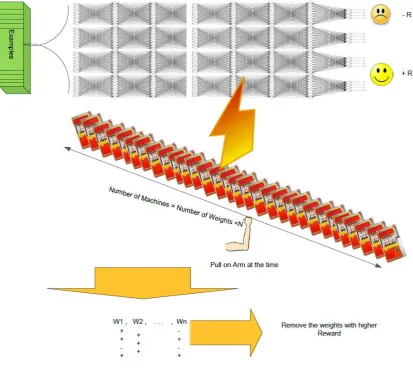
One of the most successful methods for decision making with trade-offs is known as multi-armed bandits [41-56]. Multi-multi-armed bandits provide a framework for studying the exploitation versus exploration dilemma. The scenario for multi-armed bandits involves modelling a gambler who faces a collection of slot machines and needs to select the sequence of machines to be played in order to maximize the rewards. The gambler pulls the arm of a selected machine and receives a reward or not. The goal of the gambler is to maximize the total rewards obtained during a period of playing time. A player needs to choose between an arm that gives the best reward so far (exploitation) or discovering some other arms hoping to find a better arm (exploration).

The aim of this study is to explore if multi-armed bandit algorithms can be used to decide which neurons, feature maps or weights can be removed and lead to efficient neural network models. Given this aim, the research objectives are:

1. To survey and review existing methods for pruning neural networks.

2. To research different multi-armed bandit algorithms that can be adopted for pruning deep neural networks.

3. To utilize multi-armed bandits to develop new methods for pruning deep learning models.

4. To carry out an empirical evaluation of the new multi-armed bandits pruning methods with respect to existing approaches for pruning.

Kothari [57] categorises the different types of research based on whether is it descriptive or analytical, applied or fundamental, quantitative or qualitative and conceptual or experimental. These are summarized below based on the exposition in Kothari [57].

(22)

Descriptive Research vs. Analytical Research

In descriptive research, the researcher often conducts surveys and enquiries of different kinds for the collection of data. Descriptive research is mainly employed when existing issues need to be addressed or described. This approach finds its application in the fields of social sciences and business and management studies. This method can be differentiated from other methods on the basis that the researcher cannot control the variables; as they are only responsible for reporting events of the past or present. The research projects that undertake this approach are used for the researcher to analyse the existing factors like how frequently a population changes their wardrobe, what brands people prefer, which show has the most viewers etc. All types of survey methods can be classified as descriptive research, including comparative and correlation techniques. However, analytical research is completely different from the former as the researcher has to critically evaluate the material through analysis of given data.

Applied Research vs. Fundamental Research

Research can also be classified as either applied research or fundamental research. In the former, the researcher aims to resolve an immediate problem faced by society or an organization. While, in fundamental or pure research the researcher is dedicated to formulating a theory. Fundamental research is often described as conducting a study with the sole purpose of obtaining knowledge. To give a few examples: research in which human behaviour is studied and related generalizations are made can be classified as fundamental research. Applied research is effective in resolving practical problems at hand; whereas, fundamental research works to formulate theories that will be used as a basis for further studies and have applications at present as well as for the future, and contribute to the body of scientific knowledge.

Quantitative vs. Qualitative 

(23)

Conceptual vs. Experimental (or Empirical)

Conceptual research is based on abstract ideas or theories. It is most popular among philosophers and thinkers for developing new concepts or for finding new interpretations of those that already exist. In contrast, experimental research is purely based on experiments and/or observations and not much regard is given to a system and theory. Experimental research is a data-based research, where hypotheses are formulated to be verified by observation or experiment. Data must be collected from its source directly in this type of research and standard experimentation for the simulation of desired information must be performed. The researcher is required to have a working hypothesis or guess as to the probable results for initiating this type of research. Their next responsibility is to gather data in favour of or against their hypothesis. Then comes the experimental designs stage, where the materials or subjects are manipulated to obtain the desired information that would prove or disprove the hypothesis. In this type of research, the experimenter has control over the variables being studied and the deliberate manipulation of these variables gives us the results. When a correlation between variables has to be established, empirical research must be used. It is thought that experiments or empirical studies provide the strongest evidence to prove or disprove a given hypothesis.

How to Approach Research?

(24)

predicting results under different conditions. In the qualitative approach the attitudes, opinions and behaviours are analysed subjectively.

In the field of machine learning, where this thesis sits, researchers have mainly utilized experimental and theoretical (fundamental) methods; quantitative approach; and analytical research. Most studies involving algorithm development [58] involve an empirical comparison with respect to other algorithms and utilize an experimental methodology, hence in this study also utilizes this approach. The main steps of this approach are:

1. Carrying out an in-depth literature review on the present methods and techniques to overcome the problem.

2. Design and implement a solution in mind of the problems, which involves devising novel pruning methods that have the ability to prune deep neural networks

3. Empirical evaluation: This involves carrying out many experiments to test the proposed methods.

4. Results analysis: Involves analysing and contrasting the results with similar works in the same domain. A conclusion is established from the findings. The key objective of the developed methods is achieved, with the results seen to outperform the existing works in the same field.

To achieve the desired research goal, namely to develop new algorithms for pruning using MABs that perform well, the following steps are used:

Dataset collection: Most of the modelling approaches in supervised learning fall under the category of data-driven techniques, in which a model learns from human annotation data. It is therefore important to highlight the public available data sets such as the data set from UCI Machine Learning Repository and other different recourses.

Data preparation: For the purposes of this dissertation, the dataset is assumed to be made up of a set of pairs (x, y), where x is an input example and y is a label. The dataset was subsequently divided into three folds, usually a training, validation and test fold (usual percentages could be 60%, 20%, and 20% respectively). However, if the datasets were small then cross validation was used.

(25)

mean is amongst the common pre-processing techniques. Besides using the fixed statistics to process the validation and test data, estimating these statistics on the training data is an important activity, as this appropriately simulates the deployment of the final system into a real-world application

Architecture design: For the small data sets, forward neural networks were used to build the model. Image data sets were mostly used for convolutional neural networks and temporal data sets were used with recurrent neural networks.

Optimization: The neural networks were trained and evaluated on a validation dataset. During the training, we monitor the training and validation error. Then the model with the best validation and training error was chosen.

Pruning the model: Once the model was trained then we pruned the model based on the proposed methods and other pruning methods. A preliminary review of the existing work on pruning methods, revealed the following types of methods which were used for comparison:

• Direct methods.

• Regularization and pruning based on magnitude. • Activation methods.

• First and second order derivative pruning.

Evaluation: The pruned models were evaluated one time on the test set and the accuracy is reported and compared to other pruning techniques. Non-parametric statistical methods are used to validate differences in performance between the various algorithms.

(26)

[image:26.595.86.514.69.408.2]

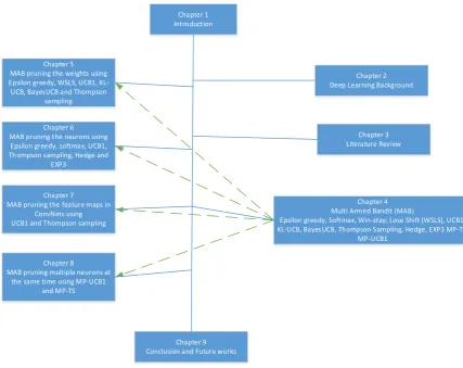
Figure 1.1: Overview of the Thesis Structure.

The following summarizes each chapter of the thesis:

Chapter 2. Deep Learning Background: This chapter describes the background and state-of-the-art deep learning models.

Chapter 3. Literature Review: This chapter begins with a brief introduction to the problem of reducing the number of parameters in deep neural networks. After a brief history, details of different kinds of pruning techniques that are identified in the literature survey are reviewed and their strengths and weaknesses presented.

Chapter 4. Multi-Armed Bandits: The literature includes several multi-armed bandit algorithms, each with different characteristics. Chapter 4 introduces the algorithms that are utilized to design and develop the new algorithms for pruning.

Chapter 5. Multi-Armed Bandits for Pruning the Weights: The multi-armed bandits described in Chapter 4 can be utilized either to develop algorithms for pruning neurons, feature maps or weights of a neural network. Chapter 5 describes the use of

Chapter 1 Introduction

Chapter 2 Deep Learning Background

Chapter 3 Literature Review

Chapter 4 Multi Armed Bandit (MAB)

Epsilon greedy, Softmax, Win-stay; Lose Shift (WSLS), UCB1, KL-UCB, BayesUCB, Thompson Sampling, Hedge, EXP3 MP-TS,

MP-UCB1 Chapter 5

MAB pruning the weights using Epsilon greedy, WSLS, UCB1, KL-UCB, BayesUCB and Thompson

sampling

Chapter 6 MAB pruning the neurons using Epsilon greedy, softmax, UCB1, Thompson sampling, Hedge and

EXP3

Chapter 7

MAB pruning the feature maps in ConvNets using UCB1 and Thompson sampling

Chapter 8

MAB pruning multiple neurons at the same time using MP-UCB1

and MP-TS

(27)

MAB methods for pruning the weights. In addition, the chapter presents implementation of MAB pruning algorithms. The implementation is used to evaluate the performance of the MAB pruning algorithms in comparison to each other as well as with existing algorithms.

Chapter 6. Multi-Armed Bandit Algorithms for Pruning the Neurons: This chapter presents the MAB algorithms for pruning neurons and presents the results from comparing the results with state of the art pruning methods.

Chapter 7. Multi-Armed Bandit Algorithms for Pruning Feature Maps: Chapter 7 presents pruning algorithms based on two MAB methods, known as UCB1 and Thompson Sampling, for pruning feature maps and their filter of convolutional layers in ConvNets. The chapter presents the results of pruning the feature maps from ConvNets and comparing the results with the well-known pruning algorithms.

Chapter 8. Multi Armed Bandit Algorithms for Pruning Multiple Neurons and Feature

Maps: The previous chapters discussed the use of MAB algorithms for pruning individual weights, neurons or feature maps. This chapter studies the ability of multiple play Thompson Sampling and UCB1 to prune multiple neurons and feature maps at the same time.

(28)

Chapter 2: Deep Learning Background 11

This chapter presents the background and technical details of different types of neural networks. First, we will begin with a conceptual overview of supervised learning which includes the objective (loss) function and regularization methods. Then, the chapter gives an introduction to optimization and back propagation. Finally, the chapter gives an introduction to feed forward neural networks, convolutional neural networks, and recurrent neural networks. The book by Goodfellow et al. [59] is recommended for a comprehensive and slower-paced overview. In addition, Karpathy [60], Bishop [61] and Abu-Mostafa et al. [62] are the main source for this chapter.

In artificial intelligent, computer programs can be used to map a function f between two spaces for example 𝑓𝑓: X→Y, where X is called an input space and Y is known an output space. For instance, in visual recognition, the space of images can be represented as the input X and the interval [0, 1] represents the Y through which the possibility of an object (like a dog) emerging somewhere in the image is indicated. As another example, in opinion mining, X

could be the sentence and Y could be the opinion of the sentence, such as liked, neutral or disliked. Traditionally, specifying or programming the function f explicitly can be difficult for tasks such as image recognition, natural language processing and automatic speech recognition. Supervised learning offers an alternative in which examples (𝑥𝑥,𝑦𝑦) ∈ 𝑋𝑋×𝑌𝑌 of the desired mapping are used to learn the mapping. For our examples, this suggests collecting a data set of images, wherein each may be marked with the absence or presence of a dog, as the same is interpreted by human beings or collecting a data set of sentences from social

2. Deep Learning Background

(29)

media and where each sentence is labelled by carrying either positive or negative meaning [60].

More formally, a data set of n examples is given by {(𝑥𝑥₁,𝑦𝑦₁), … , (𝑥𝑥_𝑛𝑛,𝑦𝑦_𝑛𝑛)}, where the independent and identically distributed (i.i.d.) samples are utilized to produce these examples from a data generating distribution 𝐷𝐷; 𝜇𝜇.𝑒𝑒. (𝑥𝑥_𝑖𝑖,𝑦𝑦_𝑖𝑖)~𝐷𝐷 for all i [60, 62].

Subsequently, we think about learning the mapping 𝑓𝑓:𝑋𝑋 → 𝑌𝑌 by looking for a set of candidate functions, where we attempt to identify the one, which is properly in line with the training examples.

In particular, a class of functions F is taken into account. Then, to measure the disagreement between a true label 𝑦𝑦_𝑖𝑖 and a predicted label 𝑦𝑦�_𝑖𝑖 = 𝑓𝑓(𝑥𝑥_𝑖𝑖) for some 𝑓𝑓 ∈ 𝐹𝐹, a scalar-valued loss function 𝐿𝐿( 𝑦𝑦�_𝑖𝑖,𝑦𝑦) is chosen. Finding out 𝑓𝑓∗ ∈ 𝐹𝐹 that minimizes the expected loss is the goal in learning and formally stated as [62]:

𝑓𝑓∗₌ _{𝑎𝑎𝑎𝑎𝑎𝑎 𝑚𝑚𝜇𝜇𝑚𝑚}

𝑓𝑓∈𝐹𝐹 𝐸𝐸(𝑥𝑥,𝑦𝑦)~𝐷𝐷𝐿𝐿(𝑓𝑓(𝑥𝑥),𝑦𝑦) (2.1)

Where argmin is argument of the minimum which the value of f for which the expected loss attains it is minimum. 𝐸𝐸₍_𝑥𝑥_,_𝑦𝑦_)~_𝐷𝐷 is the expected loss over the data generating distribution D.~ means the input data is sampled (generated) from the D. Since all the possible elements of

D are not accessible, the optimization in Equation 2.1 is intractable. Hence, the possibility cannot be evaluated or without making idealistically strong assumptions about the form of

L, D, or f, we cannot systematically streamline this process. Nonetheless, the expected loss in Equation 2.1 can be estimated with the aid of sampling and can be determined by averaging the loss over the available training data [60]:

𝑓𝑓∗ _{≈ 𝑎𝑎𝑎𝑎𝑎𝑎 𝑚𝑚𝜇𝜇𝑚𝑚} 𝑓𝑓∈𝐹𝐹

1

𝑛𝑛∑𝑛𝑛𝑖𝑖=1𝐿𝐿(𝑓𝑓(𝑥𝑥𝑖𝑖),𝑦𝑦𝑖𝑖) (2.2)

More specifically, the loss over the available training examples is optimized; however, this is hopefully a good proxy for the actual objective mentioned in Equation 2.1.

(30)

There can be problems where Equation 2.2 is optimized instead of Equation 2.1. For example, suppose a function f where each 𝑥𝑥_𝑖𝑖 in the training data is mapped to its corresponding 𝑦𝑦_𝑖𝑖, however zero is returned everywhere else. We can present this as a solution to Equation 2.2 (for any sensible loss function L, where a minimum value is attained when 𝑦𝑦= 𝑦𝑦�), but all other points in D that are not in the training set would receive a huge loss. More specifically, this function would not be expected to be generalized to all (𝑥𝑥,𝑦𝑦)~𝐷𝐷. One approach to avoiding this is to introduce a regularization term R into the loss function [60]:

𝑓𝑓∗ ₌_{𝑎𝑎𝑎𝑎𝑎𝑎 𝑚𝑚𝜇𝜇𝑚𝑚} 𝑓𝑓∈𝐹𝐹

1

𝑛𝑛∑ 𝐿𝐿(𝑓𝑓(𝑥𝑥𝑖𝑖),𝑦𝑦𝑖𝑖) + 𝜆𝜆 𝑛𝑛𝑅𝑅(𝑓𝑓) 𝑛𝑛

𝑖𝑖=1 ( 2.3)

Where 𝜆𝜆 is positive number and there are many types of regularization [63-67], and two that have been widely used are the L2 and L1 norms:

L2 norm: 𝑅𝑅(𝑓𝑓) =1

2∑ 𝑓𝑓𝑓𝑓 2

Where L2 norm is known as weight decay and is the sum of the squares of all the weights in the network

L1 norm: 𝑅𝑅(𝑓𝑓) =∑_𝑓𝑓|𝑓𝑓|.

L1 norm is the sum of the absolute values of the weights:

In the previous section, it was observed that the task of learning a model for a supervised learning problem can be reduced to solving an optimization problem having the form 𝜃𝜃∗ =

𝑎𝑎𝑎𝑎𝑎𝑎min_𝜃𝜃 𝑎𝑎(𝜃𝜃), where 𝜃𝜃 is a parameter vector and g normally amalgamates a regularization

penalty and the average loss of all examples. The following subsections present the most widely used optimization techniques in neural networks [60].

2.1.2.

Regularization

(31)

By making additional assumptions about 𝑎𝑎, the efficiency of the optimization can be enhanced [60]. Specifically, if there is no other option to use except the differentiable functions, a method known as back propagation (its details will be discussed in the next section) would be employed to compute the gradient 𝛻𝛻_𝜃𝜃𝑎𝑎. A vector of partial derivatives is referred to as the gradient, which offers the slope of 𝑎𝑎 along every dimension of 𝜃𝜃.

The gradient can be applied as a search direction. We can specifically improve 𝜃𝜃 (in the sense of attaining lower 𝑎𝑎), by adding a small amount of the negative gradient. In general, the Gradient Descent (GD) [68, 69] algorithm iterates between the following two steps:

1. The gradient is evaluated.

2. A small step is made in the direction of the negative gradient, the parameters are updated.

In general, the step size 𝜆𝜆 (also called the learning rate) is a critical parameter in Gradient Descent (GD). The optimization may not converge or even diverge, if the learning rate is too high. Moreover, the learning would become a lengthy process, if it is specified very low [60].

There are three kinds of GD based on how many samples we use to compute the gradient of the loss function [60].

Batch Gradient Descent: Batch GD computes the gradient of the loss function with respect the model’s parameters 𝜃𝜃. The following steps summarise the batch GD algorithm [68, 69]: • Estimate the gradient ∇_𝜃𝜃𝑎𝑎(𝜃𝜃) with back propagation over all training data set n

∇𝜃𝜃𝑎𝑎(𝜃𝜃) ≈ ∇𝜃𝜃�_𝑛𝑛1∑𝑛𝑛𝑖𝑖=1𝐿𝐿(𝑓𝑓𝜃𝜃(𝑥𝑥𝑖𝑖),𝑦𝑦𝑖𝑖) +𝑅𝑅(𝑓𝑓𝜃𝜃)�

• Compute the direction 𝛿𝛿𝜃𝜃 =𝜆𝜆∇_𝜃𝜃𝑎𝑎(𝜃𝜃) where 𝜆𝜆 ∈ 𝑅𝑅+(positive real number) is learning rate or step size

• Perform a parameter update 𝜃𝜃_𝑖𝑖+1 =𝜃𝜃_𝑖𝑖 − 𝛿𝛿𝜃𝜃_𝑖𝑖

One problem with batch GD occurs when there is a huge training data set (e.g. there are over 1 million training images in ImageNet). Then, these training data sets cannot fit into the memory during the learning.

(32)

Stochastic Gradient Descent (SGD): Instead of computing ∇_𝜃𝜃𝑎𝑎(𝜃𝜃)≈

∇𝜃𝜃�_𝑛𝑛1∑𝑛𝑛𝑖𝑖=1𝐿𝐿(𝑓𝑓𝜃𝜃(𝑥𝑥𝑖𝑖),𝑦𝑦𝑖𝑖) +𝑅𝑅(𝑓𝑓𝜃𝜃)� over all the training data set, SGD [28] computes over one

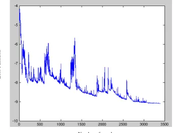
single example in the training data set and is faster than batch GD. One problem with this technique is that SGD performs frequent updates with a high variance that cause the loss function to fluctuate heavily as shown in Figure 2.1.

L

os

s F

unc

ti

on

[image:32.595.128.472.226.488.2]

Number of epochs

Figure 2.1: SGD fluctuation 2.

Mini-Batch Gradient Descent: In this method, the gradient is estimated through a small mini-batch of examples (e.g. around 200) at a time. As a result, we are enabled to perform a number of approximate updates rather than fewer exact updates. It is an approach, which has excellent functionality / working in most practical applications [70].

(33)

The computation of the update direction (Step 2 in GD) can be adjusted and modified to improve the rate of convergence. For example, a method, known as momentum [71], utilizes a proportion of the previous gradients to help maintain a consistent direction thereby often increasing the rate of convergence. The update Δ𝜃𝜃 is initially computed by updating an intermediate variable𝑣𝑣_𝑖𝑖+1=𝛾𝛾𝑣𝑣_𝑖𝑖 +𝜆𝜆∇_𝜃𝜃𝑎𝑎(𝜃𝜃) (initialized at zero). It is worth indicating that an exponentially-decaying sum of previous gradient directions is encompassed in the variable v. The following steps are the GD with momentum:

• Sample a minibatch of m examples from the training data set

• Estimate the gradient ∇_𝜃𝜃𝑎𝑎(𝜃𝜃) with back propagation over m sampling of training

data set n∇_𝜃𝜃𝑎𝑎(𝜃𝜃) ≈ ∇_𝜃𝜃�1

𝑚𝑚∑𝑚𝑚𝑖𝑖=1𝐿𝐿(𝑓𝑓𝜃𝜃(𝑥𝑥𝑖𝑖),𝑦𝑦𝑖𝑖) +𝑅𝑅(𝑓𝑓𝜃𝜃)�

• Compute the update direction 𝛿𝛿𝜃𝜃 =𝑣𝑣 where 𝑣𝑣_𝑖𝑖+1= 𝛾𝛾𝑣𝑣_𝑖𝑖 +𝜆𝜆∇_𝜃𝜃𝑎𝑎(𝜃𝜃) and 𝛾𝛾 ∈ 𝑅𝑅 (real number and practically set to 0.9) and is called momentum.

Figure 2.2 shows the difference between GD with and without momentum. Figure 2.2(a) shows the problem of GD which is that GD oscillates across the slopes of the ravine [72], while Figure 2.2(b) shows how momentum helps accelerate GD in the relevant direction.

(a) GD without momentum (b) GD with momentum

Figure 2.2: The effect of adding momentum to GD3_.

3_{http://ruder.io/optimizing-gradient-descent/index.html#fn:1}

(34)

Adagrad [73] adapts the learning to the parameters. Adagrad uses the estimate of the ﬁrst moment of the gradient (the mean). For instance, an intermediate variable r is used by Adagrad update [73], where 𝑎𝑎_𝑖𝑖+1 =𝑎𝑎_𝑖𝑖+∇_𝜃𝜃𝑎𝑎(𝜃𝜃)⨀∇_𝜃𝜃𝑎𝑎(𝜃𝜃) of sum of squared gradients (⨀ is element wise multiplication). Subsequently, the update is modulated by the second moment (the uncentered variance) like this: 𝛿𝛿𝜃𝜃 = 𝜆𝜆

𝛿𝛿+√𝑟𝑟⨀∇𝜃𝜃𝑎𝑎(𝜃𝜃), where 𝛿𝛿 is a small

number (e.g. 1𝑒𝑒−5), stopping division by zero [60]. The steps for Adagrad can be summarized as following [36]:

• Compute the update direction 𝛿𝛿𝜃𝜃 = 𝜆𝜆

𝛿𝛿+√𝑟𝑟⨀∇𝜃𝜃𝑎𝑎(𝜃𝜃) where 𝑎𝑎𝑖𝑖+1 = 𝑎𝑎𝑖𝑖 +

∇𝜃𝜃𝑎𝑎(𝜃𝜃)⨀∇𝜃𝜃𝑎𝑎(𝜃𝜃).

The main advantage of Adagrad is that it does not need to manually update the learning rate throughout the training and in most practical implementations it is to 0.01 [74, 75]. The main disadvantage of Adagrad is growth of the denominator because of accumulation of the squared gradients r. This leads the learning rate to shrink over time [76].

A running mean of the second moment is used by the RMSProp update [77] here, 𝑎𝑎_𝑖𝑖+1= ρ_r_i_{+ (1}₋ρ₎_∇_𝜃𝜃_𝑎𝑎₍_𝜃𝜃₎_⨀∇_𝜃𝜃_𝑎𝑎₍_𝜃𝜃₎, where ρ is often set to 0.99. The following steps summarize the RMSProp algorithm [36]:

2.2.3.

Adagrad

(35)

• Compute the update direction 𝛿𝛿𝜃𝜃= 𝜆𝜆

𝛿𝛿+√𝑟𝑟⨀∇𝜃𝜃𝑎𝑎(𝜃𝜃) where 𝑎𝑎𝑖𝑖+1 =ρri+ (1−

ρ₎_∇_𝜃𝜃_𝑎𝑎₍_𝜃𝜃₎_⨀∇_𝜃𝜃_𝑎𝑎₍_𝜃𝜃₎.

Adam adapts the estimation of both the ﬁrst and second moments [78] and it can be seen as a mix of RMSProp with momentum. The first moment of the gradients 𝑚𝑚_𝑔𝑔 (𝑚𝑚_𝑔𝑔_,_𝑡𝑡is 𝑚𝑚_𝑔𝑔 at time t or the current time) is computed by 𝑚𝑚_𝑔𝑔_,_𝑡𝑡+1=𝛽𝛽₁𝑚𝑚_𝑔𝑔_,_𝑡𝑡+ (1− 𝛽𝛽₁)∇_𝜃𝜃𝑎𝑎(𝜃𝜃) and the second moment of the gradients 𝑣𝑣_𝑔𝑔 (𝑣𝑣_𝑔𝑔_,_𝑡𝑡𝜇𝜇𝑖𝑖𝑣𝑣_𝑔𝑔𝑎𝑎𝑎𝑎𝑎𝑎𝜇𝜇𝑚𝑚𝑒𝑒𝑎𝑎) is computed by 𝑣𝑣_𝑔𝑔_,_𝑡𝑡+1= 𝛽𝛽₂𝑣𝑣_𝑔𝑔_,_𝑡𝑡+ (1− 𝛽𝛽2)(∇𝜃𝜃𝑎𝑎(𝜃𝜃))2 where 𝛽𝛽1and 𝛽𝛽2 are close to one and practically are set to 0.9 and 0.999

respectively [78]. Subsequently, the update is modulated by these first and second moments thus: 𝛿𝛿𝜃𝜃= 𝜆𝜆

𝛿𝛿+√𝑣𝑣�𝑚𝑚�, where 𝛿𝛿 is a small number (e.g. 1𝑒𝑒−5) where 𝑚𝑚� = 𝑚𝑚𝑔𝑔

1−𝛽𝛽1 and 𝑣𝑣�=

𝑣𝑣𝑔𝑔

1−𝛽𝛽2.

The following steps summarizes the Adam algorithm [37]:

data set n ∇_𝜃𝜃𝑎𝑎(𝜃𝜃) ≈ ∇_𝜃𝜃�1

• Compute the update direction 𝛿𝛿𝜃𝜃= 𝜆𝜆

𝛿𝛿+√𝑣𝑣�𝑚𝑚�, where 𝛿𝛿 is a small number (e.g. 1𝑒𝑒−8)

where 𝑚𝑚� = 𝑚𝑚𝑔𝑔

𝑣𝑣𝑔𝑔

1−𝛽𝛽2

The previous section shows that if the gradient of the loss function can be estimated, then GD can be used to reduce it. Back propagation [1, 79-81] is a process where gradients of scalar valued functions are efficiently computed based on their inputs. From calculus, a recursive application of the chain rule is none other than the back propagation algorithm. Remember that 𝑎𝑎 is the main function to calculate the gradients. This function takes the parameters θ and the data set of examples (𝑥𝑥_𝑖𝑖,𝑦𝑦_𝑖𝑖) as input.

2.2.5.

Adam

(36)

To understand back propagation, we assume there is an input vector 𝑥𝑥₀, which is converted through a series of functions 𝑥𝑥_𝑖𝑖 = 𝑓𝑓_𝑖𝑖(𝑥𝑥_𝑖𝑖−1) where i =1,...,k and the last 𝑥𝑥_𝑘𝑘 is a scalar. Then the following steps summarize the back propagation algorithm [60]:

• Compute forward propagation given the input 𝑥𝑥₀. So 𝑥𝑥₁ = 𝑓𝑓₁(𝑥𝑥₀), …, 𝑥𝑥_𝑖𝑖 = 𝑓𝑓_𝑖𝑖(𝑥𝑥_𝑖𝑖−1), …, 𝑥𝑥_𝑘𝑘 =𝑓𝑓_𝑘𝑘(𝑥𝑥_𝑘𝑘−1) where 𝑓𝑓_𝑖𝑖 are activation functions.

• Using the chain rule, compute the gradient 𝜕𝜕𝑥𝑥𝑘𝑘

𝜕𝜕𝑥𝑥0 that will include computing the

gradient of all intermediate transformations. These gradients are known as a Jacobian matrix and each transform is given by 𝜕𝜕𝑥𝑥_𝑖𝑖⁄𝜕𝜕𝑥𝑥_𝑖𝑖−1.

• Then, the final gradient is given by 𝜕𝜕𝑥𝑥𝑘𝑘

𝜕𝜕𝑥𝑥0 =∏ 𝜕𝜕𝑥𝑥𝑖𝑖⁄𝜕𝜕𝑥𝑥𝑖𝑖−1

𝑘𝑘

𝑖𝑖=1 . This matrix product of

all the Jacobians is used by the GD algorithm as an estimate of the gradient ∇_𝜃𝜃𝑎𝑎(𝜃𝜃).

Example: To understand back propagation and GD, consider this example: Assume we have a data set that contains two features 𝑥𝑥₀ and 𝑥𝑥₁ and one output 𝑦𝑦 as described in the Table 2-1.

X0 X1 y

0 1 1

2 1 4

1 0 2

1 1 1

Table 2-1: Example of a small data set where X0 and X1 are features and y is the output.

(37)

Chapter 2: Deep Learning Background 20 x0 x1 Mul(*) Mul(*) Add(+) 1 1=−

w

1 0= w 1 2= w 2 3= w x0 Mul(*) Mul(*)

Add(+) Output f

1

1=− w 1 0= w 1 2= w 2 3= w x1 Mul(*) Mul(*)

[image:37.595.227.381.380.559.2]

(a) Graph with 3 nodes, external inputs, and outputs (b) The graph unfolded to explain the operation

Figure 2.3: Example of graph of multiple nodes.

The following steps represent the GD and back propagation in Figure 2.3:

The first step: For simplicity, we will use SGD which applies GD with one example from the training data set that is shown in Table 2-1.

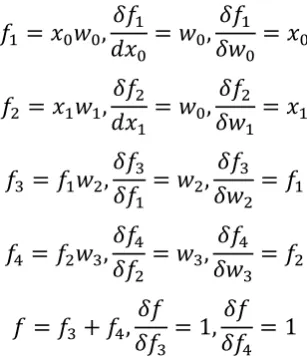
The second step: Compute forward propagation as following:

𝑓𝑓1 = 𝑥𝑥0𝑤𝑤0,_{𝑑𝑑𝑥𝑥}𝛿𝛿𝑓𝑓1

0 = 𝑤𝑤0,

𝛿𝛿𝑓𝑓1

𝛿𝛿𝑤𝑤0 =𝑥𝑥0

𝑓𝑓2 = 𝑥𝑥1𝑤𝑤1,_{𝑑𝑑𝑥𝑥}𝛿𝛿𝑓𝑓2

1 = 𝑤𝑤0,

𝛿𝛿𝑓𝑓2

𝛿𝛿𝑤𝑤1 =𝑥𝑥1

𝑓𝑓3 =𝑓𝑓1𝑤𝑤2,𝛿𝛿𝑓𝑓_{𝛿𝛿𝑓𝑓}3 1 = 𝑤𝑤2,

𝛿𝛿𝑓𝑓3

𝛿𝛿𝑤𝑤2 =𝑓𝑓1

𝑓𝑓4 =𝑓𝑓2𝑤𝑤3,𝛿𝛿𝑓𝑓_{𝛿𝛿𝑓𝑓}4 2 =𝑤𝑤3,

𝛿𝛿𝑓𝑓4

𝛿𝛿𝑤𝑤3 = 𝑓𝑓2

𝑓𝑓= 𝑓𝑓3+𝑓𝑓4,_{𝛿𝛿𝑓𝑓}𝛿𝛿𝑓𝑓

3 = 1,

𝛿𝛿𝑓𝑓 𝛿𝛿𝑓𝑓4 = 1

Given the third example in the data set and after substituting the values from Table 2-1 and Figure 2.3 we get the following:

𝑓𝑓1 = 1×1 = 1

𝑓𝑓2 = 1×−1 = −1

𝑓𝑓3 = 1×1 = 1

𝑓𝑓4 =−1×2 =−2

𝑓𝑓= 1 + (−2) =−1

(38)

𝐿𝐿=1_{2 (}𝑦𝑦 − 𝑓𝑓)2 ₌1

2 (1−(−1))2 = 2 Computing the Jacobian matrix using chain role gives:

𝛿𝛿𝐿𝐿 𝛿𝛿𝑓𝑓=−2 𝛿𝛿𝐿𝐿

𝛿𝛿𝑓𝑓4 =

𝛿𝛿𝐿𝐿 𝛿𝛿𝑓𝑓

𝛿𝛿𝑓𝑓

𝛿𝛿𝑓𝑓4 = −2∗1 =−2

𝛿𝛿𝐿𝐿 𝛿𝛿𝑓𝑓3 =

𝛿𝛿𝑓𝑓

𝛿𝛿𝑓𝑓3 = −2∗1 =−2

𝛿𝛿𝑓𝑓 𝛿𝛿𝑓𝑓3

𝛿𝛿𝑓𝑓3

𝛿𝛿𝑓𝑓1 =−2∗1 = −2

𝛿𝛿𝐿𝐿 𝛿𝛿𝑤𝑤2 =

𝛿𝛿𝑓𝑓3

𝛿𝛿𝑤𝑤2 =−2∗1 = −2

𝛿𝛿𝐿𝐿 𝛿𝛿𝑓𝑓 𝛿𝛿𝑓𝑓 𝛿𝛿𝑓𝑓3 𝛿𝛿𝑓𝑓3 𝛿𝛿𝑓𝑓1 𝛿𝛿𝑓𝑓1

𝛿𝛿𝑤𝑤0 = −2∗1∗1 = −2

𝛿𝛿𝑓𝑓4

𝛿𝛿𝑓𝑓2 =−2∗2 =−4

𝛿𝛿𝑓𝑓4

𝛿𝛿𝑤𝑤3 =−2∗(−1) = 2

𝛿𝛿𝐿𝐿 𝛿𝛿𝑓𝑓 𝛿𝛿𝑓𝑓 𝛿𝛿𝑓𝑓4 𝛿𝛿𝑓𝑓4 𝛿𝛿𝑓𝑓2 𝛿𝛿𝑓𝑓2

𝛿𝛿𝑤𝑤1 = −2∗2∗1 =−4

In this example, we assume the parameters of the graph only Ws then ∇_𝜃𝜃𝑎𝑎(𝜃𝜃) =∇_𝑤𝑤𝑎𝑎(𝑤𝑤):

∇𝜃𝜃𝑎𝑎(𝜃𝜃) =∇𝑤𝑤𝑎𝑎(𝑤𝑤) =

⎣ ⎢ ⎢ ⎢ ⎡𝛿𝛿𝐿𝐿 𝛿𝛿𝑤𝑤0 𝛿𝛿𝐿𝐿 𝛿𝛿𝑤𝑤1 𝛿𝛿𝐿𝐿 𝛿𝛿𝑤𝑤2 𝛿𝛿𝐿𝐿 𝛿𝛿𝑤𝑤3⎦⎥

⎥ ⎥ ⎤

= �−₋2₂ −₂4�

The next step, after computing ∇_𝜃𝜃𝑎𝑎(𝜃𝜃) using back propagation involves updating the parameters. However, as described in Section 2.2, there are different GD algorithms and the following presents how each one of them updates the parameters.

Updates using SGD

First, we will start with vanilla SGD. The third step of the algorithm is as following:

𝛿𝛿𝜃𝜃=𝜆𝜆∇𝜃𝜃𝑎𝑎(𝜃𝜃) where the learning rate 𝜆𝜆 = 0.1 then

𝛿𝛿𝑤𝑤𝑖𝑖+1 =𝛿𝛿𝜃𝜃𝑖𝑖+1= 𝜆𝜆∇𝑤𝑤,𝑖𝑖𝑎𝑎(𝜃𝜃) = 0.1∗ �−₋₂2 −₂4�=�−₋0.2_0.2 −_0.20.4�

(39)

𝑤𝑤𝑖𝑖+1= 𝜃𝜃𝑖𝑖+1= 𝜃𝜃𝑖𝑖 − 𝛿𝛿𝜃𝜃𝑖𝑖 =𝑤𝑤𝑖𝑖 − 𝛿𝛿𝑤𝑤𝑖𝑖 =�1₁ −₂1� − �−₋0.2_0.2 −_0.20.4�=�1.2_1.2 −_1.80.6�

GD with momentum at this iteration will give the same result as GD because of 𝑣𝑣_𝑖𝑖+1=

𝛾𝛾𝑣𝑣𝑖𝑖 +𝜆𝜆∇𝜃𝜃𝑎𝑎(𝜃𝜃) and at the beginning 𝑣𝑣 = 0. Then the new 𝑣𝑣𝑖𝑖+1= 𝛾𝛾𝑣𝑣𝑖𝑖 +𝜆𝜆∇𝜃𝜃𝑎𝑎(𝜃𝜃) = 0∗

0.9 +𝜆𝜆∇𝜃𝜃𝑎𝑎(𝜃𝜃) =𝜆𝜆∇𝜃𝜃𝑎𝑎(𝜃𝜃) but after this iteration, 𝑣𝑣 will affect the update.

Updates using Adagrad

The following GD is Adagrad, we compute the update direction 𝛿𝛿𝜃𝜃= 𝜆𝜆

𝛿𝛿+√𝑟𝑟⨀∇𝜃𝜃𝑎𝑎(𝜃𝜃) where

𝑎𝑎𝑖𝑖+1= 𝑎𝑎𝑖𝑖+∇𝜃𝜃𝑎𝑎(𝜃𝜃)⨀∇𝜃𝜃𝑎𝑎(𝜃𝜃) and r initializes at 0 then

𝑎𝑎𝑖𝑖+1=𝑎𝑎𝑖𝑖 +∇𝜃𝜃𝑎𝑎(𝜃𝜃)⨀∇𝜃𝜃𝑎𝑎(𝜃𝜃) = 0 +�−₋₂2 −₂4� ⨀ �−₋2₂ −₂4�=�4 16_{4 4}�

Then

𝛿𝛿𝜃𝜃= _{𝛿𝛿+√𝑟𝑟}𝜆𝜆 ⨀∇𝜃𝜃𝑎𝑎(𝜃𝜃) =𝛿𝛿𝜃𝜃= 0.1

0.00005+��4 16_{4 4 �}⨀ �−

2 −4

−2 2 �=�−−0.0250.025 −0.0250.006�

Then, perform a parameter update

𝜃𝜃𝑖𝑖+1 =𝜃𝜃𝑖𝑖−_{𝛿𝛿+√𝑟𝑟}𝜆𝜆 ⨀∇𝜃𝜃,𝑖𝑖𝑎𝑎(𝜃𝜃) =�1₁ −₂1� − �−₋0.025_0.025 −_0.0250.006�= �1.025_1.025 −_1.980.99�

Updates using RMSProp

The next GD is RMSProp, we compute the update direction 𝛿𝛿𝜃𝜃 = 𝜆𝜆

𝛿𝛿+√𝑟𝑟⨀∇𝜃𝜃𝑎𝑎(𝜃𝜃) where

𝑎𝑎𝑖𝑖+1= ρ𝑎𝑎𝑖𝑖+ (1−ρ)∇𝜃𝜃𝑎𝑎(𝜃𝜃)⨀∇𝜃𝜃𝑎𝑎(𝜃𝜃) and 𝑎𝑎𝑖𝑖 initializes at 0 then

𝑎𝑎𝑖𝑖+1= ρri+ (1−ρ)∇𝜃𝜃𝑎𝑎(𝜃𝜃)⨀∇𝜃𝜃𝑎𝑎(𝜃𝜃) = 0.99∗0 + (1−0.99)∗

�−₋₂2 −₂4� ⨀ �−₋2₂ −₂4�= �0.04 0.16_{0.04 0.04}� Then

𝛿𝛿𝜃𝜃= _{𝛿𝛿+√𝑟𝑟}𝜆𝜆 ⨀∇𝜃𝜃𝑎𝑎(𝜃𝜃) = 0.1

0.00005+��0₀._.04 0_{04 0}._.16_04�⨀ �−

2 −4

−2 2 �= �−−0.2490.249 −0.2500.063�

Then, perform a parameter update

(40)

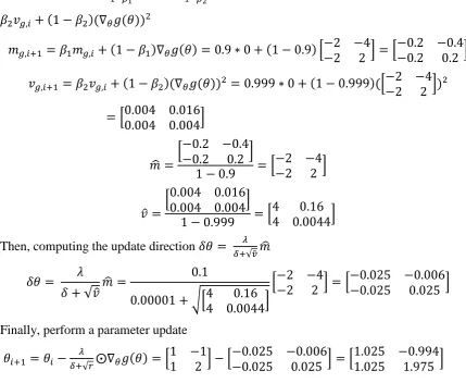
Updates using Adam

The last GD is Adam, we compute the update direction 𝛿𝛿𝜃𝜃= 𝜆𝜆

𝛿𝛿+√𝑣𝑣�𝑚𝑚�, where 𝛿𝛿 is a small

number where 𝑚𝑚� = 𝑚𝑚𝑔𝑔

𝑣𝑣𝑔𝑔

1−𝛽𝛽2, 𝑚𝑚𝑔𝑔,𝑖𝑖+1 =𝛽𝛽1𝑚𝑚𝑔𝑔,𝑖𝑖 + (1− 𝛽𝛽1)∇𝜃𝜃𝑎𝑎(𝜃𝜃) and 𝑣𝑣𝑔𝑔,𝑖𝑖+1 = 𝛽𝛽2𝑣𝑣𝑔𝑔,𝑖𝑖+ (1− 𝛽𝛽2)(∇𝜃𝜃𝑎𝑎(𝜃𝜃))2

𝑚𝑚𝑔𝑔,𝑖𝑖+1 =𝛽𝛽1𝑚𝑚𝑔𝑔,𝑖𝑖 + (1− 𝛽𝛽1)∇𝜃𝜃𝑎𝑎(𝜃𝜃) = 0.9∗0 + (1−0.9)�−₋2₂ −₂4�=�−₋0.2_0.2 −_0.20.4�

𝑣𝑣𝑔𝑔,𝑖𝑖+1=𝛽𝛽2𝑣𝑣𝑔𝑔,𝑖𝑖+ (1− 𝛽𝛽2)(∇𝜃𝜃𝑎𝑎(𝜃𝜃))2 = 0.999∗0 + (1−0.999)(�−₋₂2 −₂4�)2

=�0.004 0.016_{0.004 0.004}�

𝑚𝑚� =�−

0.2 −0.4

−0.2 0.2 �

1−0.9 = �−−22 −24�

𝑣𝑣�= �

0.004 0.016 0.004 0.004�

1−0.999 = �44 0.00440.16 � Then, computing the update direction 𝛿𝛿𝜃𝜃 = 𝜆𝜆

𝛿𝛿+√𝑣𝑣�𝑚𝑚�

𝛿𝛿𝜃𝜃= 𝜆𝜆

𝛿𝛿+√𝑣𝑣�𝑚𝑚�=

0.1

0.00001 +��4_{4 0.0044}0.16 �

�−₋2₂ −₂4�=�−₋0.025_0.025 −_0.0250.006�

Finally, perform a parameter update

𝜃𝜃𝑖𝑖+1 =𝜃𝜃𝑖𝑖−_{𝛿𝛿+√𝑟𝑟}𝜆𝜆 ⨀∇𝜃𝜃𝑎𝑎(𝜃𝜃) =�₁1 −₂1� − �−₋_0.0250.025 −_0.0250.006�=�1.025_1.025 −_1.9750.994�

Finally, from the previous example, we can notice that SGD has less hyperparameters while Adam has the most.

[image:40.595.85.515.159.511.2]

In the previous sections, it was observed that arbitrary differentiable functions f can be defined, which map the inputs x to predicted outputs 𝑦𝑦�, and that a GD procedure can be used to optimize a differentiable loss function. The function f, which has been left unspecified until now, will now be discussed.