Application of complex network principles to key station identification in railway network efficiency analysis

p r i n ci pl e s t o k e y s t a ti o n

id e n tific a ti o n i n r a il w a y n e t w o r k

e ffici e n c y a n a ly si s

Wa n g , L, An, M , Ji a, L a n d Qi n , Y

h t t p :// dx. d oi.o r g / 1 0 . 1 1 5 5 / 2 0 1 9 / 1 5 7 4 1 3 6

T i t l e

Ap plic a ti o n of c o m p l ex n e t w o r k p r i n ci pl e s t o k e y s t a ti o n

id e n tific a tio n i n r a il w a y n e t w o r k effici e n c y a n a ly si s

A u t h o r s

Wa n g , L, An, M , Jia, L a n d Qi n, Y

Typ e

Ar ticl e

U RL

T hi s v e r si o n is a v ail a bl e a t :

h t t p :// u sir. s alfo r d . a c . u k /i d/ e p ri n t/ 5 3 4 1 4 /

P u b l i s h e d D a t e

2 0 1 9

U S IR is a d i gi t al c oll e c ti o n of t h e r e s e a r c h o u t p u t of t h e U n iv e r si ty of S alfo r d .

W h e r e c o p y ri g h t p e r m i t s , f ull t e x t m a t e r i al h el d i n t h e r e p o si t o r y is m a d e

f r e ely a v ail a bl e o nli n e a n d c a n b e r e a d , d o w nl o a d e d a n d c o pi e d fo r n o

n-c o m m e r n-ci al p r iv a t e s t u d y o r r e s e a r n-c h p u r p o s e s . Pl e a s e n-c h e n-c k t h e m a n u s n-c ri p t

fo r a n y f u r t h e r c o p y ri g h t r e s t r i c ti o n s .

Research Article

Application of Complex Network Principles to Key Station

Identification in Railway Network Efficiency Analysis

Li Wang ,

Min An ,

Limin Jia ,

and Yong Qin

1_{School of Traffic and Transportation, Beijing Jiaotong Univeristy, Beijing 100044, China}

2_{School of Science, Engineering and Environment, University of Salford, Manchester M5 4WT, UK}

3_{Rail Traffic Control and Safety State Key Laboratory, Beijing Jiaotong University, Beijing 100044, China}

Correspondence should be addressed to Min An; [email protected]

Received 31 January 2019; Revised 27 July 2019; Accepted 27 August 2019; Published 2 December 2019

Academic Editor: Paola Pellegrini

Copyright © 2019 Li Wang et al. This is an open access article distributed under the Creative Commons Attribution License, which permits unrestricted use, distribution, and reproduction in any medium, provided the original work is properly cited.

Network efficiency analysis becomes important in railways in order to contribute towards improving the safety and capacity of the rail network, making rail travel more attractive for passengers, and improving industry practice and informing policy development. However, a physical railway network structure is a complicated system, and the operation, maintenance, and management of such a network is a difficult task which may be affected by many influential factors. By using efficiency analysis technology for a railway network, combining physical structure with operation functions can help railway industry to optimize the railway network while improving its efficiency and reliability. This paper presents a new methodology based on complex network principles that combines the physical railway structure with railway operation strategy for a railway network efficiency analysis. In this method, two network models of railway physical and train flow networks are developed for the identification of key stations in the railway network based on network efficiency contribution in which the terms of degree, strength, betweenness, clustering coefficient, and a comprehensive factor are taken into consideration. Once the key stations have been identified and analysed, the railway network efficiency is then studied on the basis of selective and random modes of the station failures. A case study is presented in this paper to demonstrate the application of the proposed methodology. The results show that the identified key stations in the railway network play an important role in improving the overall railway network efficiency, which can provide useful information to railway designers, engineers, operators and maintainers to operate and maintain railway network effectively and efficiently.

1. Introduction

In comparison with road transportation, railways are by far one of the safest means of ground transportation, especially for their passengers and employees. However, there are some issues involved in both maintaining this position in reality and sustaining the public perception of railway safety excellence. The railway now finds itself in a situation where actual and perceived safeties are real issues, to be dealt with in a new public culture of rapid change, short-term pressures, and instant communications [1–3]. However, operation and main-tenance of railway networks are becoming difficult, particu-larly, it is related to railway network efficiency, reliability, and safety. For example, if a key station fails to operate in a railway network, it would affect the overall railway network transpor-tation efficiency. A stranspor-tation failure to operate can be classified into physical failures of the railway physical network such as

presents a new methodology to analyse the efficiency of the railway networks using complex network principles for the key station identification, in which railway network efficiency is evaluated based on station failure modes. This will provide useful method and information to the industry in the design, operation, and maintenance of the railway network effectively and efficiently.

In the context of the network theory, a complex network can be defined as a graph that is composed of relatively many mutually related nodes including structural and functional relations, and it could also be defined as a network that has nonobservable topological features that do not arise in simple networks such as random ones but often occur in graph mod-els of real systems [9]. A railway network can be classified as a complex network and investigated through complex network analysis [4, 5]. Complex network anlaysis has been successfully applied to analyse the efficiency of networks, for example, a biology network [10], a research cooperating network [11, 12], an electricity supply system [13], a traffic network [4, 14], and even an Internet network [15]. Dey et al. [16] successfully applied complex network theory to analyse safety and relia-bility of topology impact on the propagation of cascading failure in a national power grid. Zio and Sansavini [17] also applied complex network method for modelling interdepend-ent network systems in order to idinterdepend-entify cascade-safe operat-ing margins. These researchers have developed various network analysis models and also studied the structural char-acteristics of the networks including system indicators such as node degree, length of the path, and clustering coefficient, in which the complex network vulnerability can be analysed in the selective and random node failure modes [18–21]. In the literature, some of the studies have also been conducted to investigate characteristics of transportation networks based on complex network theory. Xu et al. [22] studied urban bus transport systems, Porta et al. [23] and Wang et al. [7] looked at insight of urban street networks, Bagler [24] studied airline network, and Dall’Asta et al. [25] investigated USA airline net-work. Guidotti et al. [26] proposed a probabilistic methodol-ogy to quantify the network reliability based on current network efficiency and a measure of connectivity, i.e., eccen-tricity and heterogeneity. This method was applied to analyse a highway transportation network reliability. Qian et al. [27] developed a cascading failure model of the complex network to simulate the road traffic status by using the delay of the time, incident dissipation factor and load capacity. Chen et al. [28] presented a particle swarm optimization (PSO) algorithm to optimize the invulnerability of China railway traffic network by introducing the concept of the edge to the network. The results produced from these researches provide useful infor-mation for maintaining and operating of the complex road and airspace transportation networks.

Because a railway network is a complex network that is also suitable to be examined by using complex network prin-ciples. Lin et al. [29] and Li et al. [8] studied China’s high-speed rail network as a complex system and analysed network safety and reliability based on complex network theory. Ouyang et al. [5] also applied complex network theory to study the perfor-mance and vulnerability of railways under various types of attacks and hazards. The complex network theory has been

widely applied to the reliability and safety analysis of the com-plex networks and has also been used in railway network reli-ability analysis. However, these studies are limited to properties of the physical networks, and the railway operation functions are neglected in their analyses. It is essential to develop new methods and models to take not only the characteristics of physical railway network, but also the operation functions into considerationl in this case, train flow network needs to be integrated into the network efficiency analysis process in order to obtain reliable results.

This paper presents a new methodology to analyse railway network efficiency that combines characteristics of railway physical network with the functions of train flow network. In other words, the proposed method considers not only the physical network topologies such as degree and clustering coefficient, but also the dynamic operation parameters such as train running paths, stop-schedules, and service frequen-cies. The proposed method can be used to identify the key stations in the network and analyse railway network efficiency based on selective and random failures of stations, which pro-vides a useful method and more reliable and accurate infor-mation to railway designers, engineers, operators, and maintainers for operating and maintaining railway network effectively and efficiently.

This paper is organised into the following sections. After the introduction, Section 2 presents the development of rail-way physical network (RPN) and train flow network (TFN) and considerations in the RPN and TFN are discussed more detailed. Specific terms in mathematics are defined in Section 3, which will form the basis of the proposed method using complex network principles for key station identification in the railway network. Section 4 describes a new proposed network efficiency analysis method. A case study of a high-speed rail network efficiency analysis is presented in Section 5 to demonstrate the application of the proposed method, and recommendations are given in this section for improvement of railway network at planning, operation and maintenance in order to satisfy the railway network efficiency requirement. Finally, conclusions are given in Section 6.

2. Development of Railway Physical Network

(RPN) and Train Flow Network (TFN)

A new approach for the analysis of network efficiency is pro-posed, which combines the RPN with the TFN in order to consider network structure properties together with network operation functions in the analysis process. The RPN considers the physical connecting properties in the network and pro-vides constraints to the TFN. The RFN takes train service plan and the operation functions of TFN into consideration. The proposed railway network efficiency analysis process includes three steps, i.e., development of railway network efficiency model, identification of key station indices, station ranking, and network efficiency analysis as shown in Figure 1.

Key station identification indices can be obtained by evaluat-ing the importance of the stations in a TFN. Stations in the RPN can be ranked based on the evaluated importance of each station. Once key stations are identified, the key station iden-tification indices are then used to analyse network efficiency by the choice of failure modes of stations or the random selec-tion of failure modes of staselec-tions in the railway network.

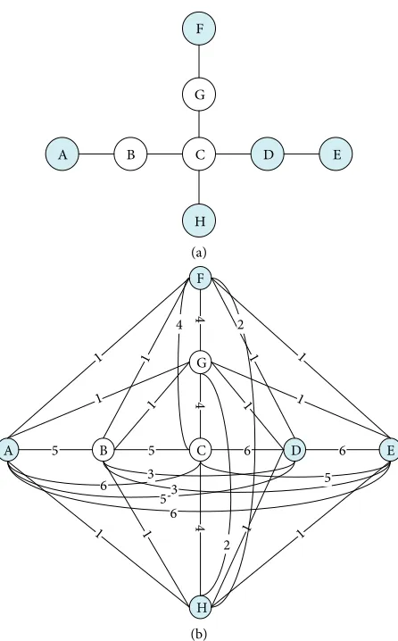
2.1. Railway Physical Network (RPN). The stations can be considered as nodes, and the connection between any two stations can be expressed as an edge in the RPN [7, 16, 22, 24]. For example, Figure 2(a) shows a simple RPN in which 8 stations are connected by two rail lines, i.e., A-B-C-D-E (5 stations) and F-G-C-H (4 stations). The station C is a junction station, and the dark nodes show that these stations are terminal stations that can be as original or destination stations of the trains. The RPN can be expressed as 𝐺𝑔= (𝑉𝑔, 𝐸𝑔), where 𝑉𝑔 is a set of railway stations in the network, and 𝐸𝑔 is a set of rail tracks. The

RPN presents the physical connectivity among the stations in the RPN in which takes the track length, section capacity and station capacity into consideration. The RPN can be used to analyse transportation capacity constraints for train service plan.

2.2. Train Flow Network (TFN). As the stations are represented as nodes in the RPN, if a train has been scheduled to be operated between two stations, this will produce one edge between these two stations as shown in Figure 2(b). The numbers of trains scheduled to stop at any two connected stations determine the weight of edge between the two stations [4]. The total number of edges can be calculated by 𝐶2

𝑛= 𝑛 × (𝑛 − 1)/2 and 𝑛 denotes a train that has a total number of stations to stop as

scheduled. For example, Figure 2(b) shows 8 stations that are connected by 28 edges, i.e., 𝐶2

8= (8 × 7)/2 = 28 between two stations based on the proposed train service plan as shown in Figure 3. The number on each edge presents frequency of trains, for example, number of 5 on edge A to C presents that 5 trains are scheduled running on this edge and stop at station A and C as shown in Figure 2(b). The TFN can be expressed as 𝐺𝑡 = (𝑉𝑡, 𝐸𝑡), where 𝑉𝑡 is the set of stations that any train can

stop at these stations, and 𝐸𝑡 is a set of edges that creates any

two stops at any stations in the RPN. Therefore, the TFN can be developed based on train service plan in which the train stop schedule creates the edges in the RPN, and frequency of trains determines the weight of the edge. Obviously, if the frequency of trains running on an edge is high, the weight of this edge is high.

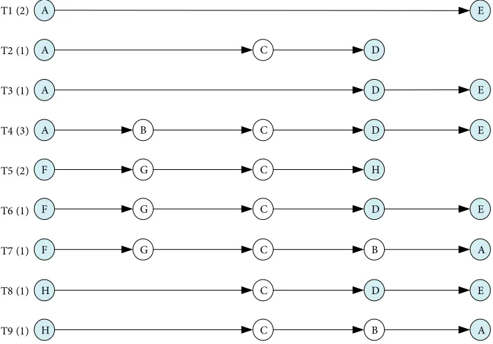
2.3. RPN and TFN Considerations. As described earlier in this paper, the RPN can be improved by taking the train service plan into consideration to produce the TFN. For example, Figure 3 shows a proposed train service plan which includes 9 stop-schedules, i.e., T1, T2, …,T9 and frequencies of trains are 2, 1, 1, 3, 2, 1, 1, 1, and 1, respectively. The nodes as shown in Figure 3 for each stop-schedule means that a train stops at these stations, for example, the stop-schedule of T4(3)

• Degree centrality (DC) • Strength centrality (SC) • Betweenness centrality (BC) • Cluster coefficient (CC)

Physical topology • Track length • Section capacity • Station capacity

Physical topology Operation strategies • Train running routes • Stop-schedules • Service frequencies Improved

based on service plan Railway network models

Train flow network

Key station identification indices

Comprehensive Factor (CF) Railway physical network

Based on key station identification indices (DC, SC, BC, CC, FF)

Station ranking

Selective mode Random mode

Network efficiency analysis

Figure 1: Railway network efficiency analysis process.

A B C D E

F

G

H (a)

A 5 B 5 C 6 D 6 E

F

G

H

4

4

4

5 6

6 3 ₃ 5

4 2

2 1

1 1

1

1 1 1 ₁

1 1

1

1

(b)

each station in the railway network, which are described as below.

3.1. Degree Centrality (DC). Assume 𝑣𝑖 denotes the 𝑖th node in the TFN, the DC of a node 𝑣𝑖 is the number of the connections

between 𝑣𝑖 and other nodes in the RPN, which describes the

physical connective influence of a node by the number of its neighbour nodes. For example, the DC of Node A is 7 (i.e., 5 + 1 + 1 = 7) as shown in Figure 2(b), which means that 7 Nodes of B, C, D, F, E, G, and H are connected to Node A directly. The DC 𝑘𝑖 of a node 𝑣𝑖 in the TFN can be defined as

where 𝑘𝑖 is the DC of a node, 𝑁 is the number of the nodes in

the RPN, and 𝑛𝑖,𝑗 is a variable of 0 or 1, i.e., if there is a con-nection between nodes 𝑣𝑖 and 𝑣𝑗, then 𝑛𝑖,𝑗= 1, otherwise,

𝑛𝑖,𝑗= 0. If a node in the TFN is connected with more edges, it

will have a large value of DC 𝑘𝑖. In other words, the DC of a node describes the reachability of the station.

3.2. Strength Centrality (SC). In the TFN, some of the edges are more important than others that depend on weights of edges. The weight of an edge presents the importance of this edge in the TFN in which it depends on frequencies of train service running on this edge, i.e., the more frequently the edge is used by trains, the more important it is. In this study, the SC is used to describe the weight of each node. For example, the SC of Node A is 25 (5 + 6 + 5 + 6 + 1 + 1 + 1 = 25) as shown in Figure 2(b). Assume SC 𝑠𝑖 of a node 𝑣𝑖 is the sum of the weights of

the edges between 𝑣𝑖 and other nodes, and it can be defined as (1) 𝑘𝑖=

𝑁

∑

𝑗=1𝑛𝑖,𝑗,

(2)

𝑠𝑖= 𝑁

∑

𝑗=1𝑤𝑖,𝑗,

indicates that 3 trains have a same stop-schedule with different departure times, and all of these 3 trains will stop at stations of A, B, C, D, and E. Based on the proposed train service plan, the TFN can be produced as shown in Figure 3 in which train service plan has been taken into consideration.

As can be seen from Figure 2(b), the edge between nodes A and B is created by stop-schedules of T4, T7, and T9 as shown in Figure 3, and the weight of edge is the sum of fre-quencies of these three stop-schedules, i.e., 3 + 1 + 1 = 5. It should be noted that there is an edge between nodes F and C in TFN as shown in Figure 2(b), although there is not a direct connection between F and C in RPN as shown in Figure 2(a). However, the edge between nodes F and C in TFN is created by stop-schedules of T5, T6, and T7 as shown in Figure 3, and the edge weight is the sum of frequencies of these three stop-schedules, i.e., 2 + 1 + 1 = 4 as shown in Figure 2(b). Similarly, other edges based on stop-schedules can be pro-duced, and the weights of edges in TFN can be calculated. In this case, the railway network physical topology in the RPN and the operation strategies such as train running routes, orig-inal stations and destination stations, stop-schedules, and service frequencies can be considered together to produce the TFN by taking the relations and weights of edges into account.

3. Factors Used in Key Station Identification

Analysis

As described in Section 2, the TFN can be developed based on the RPN by taking train service plan into consideration. Key station identification indices can be then calculated based on complex network principles [30], including degree central-ity (DC), strength centralcentral-ity (SC), betweenness centralcentral-ity (BC), clustering coefficient (CC), and comprehensive factor (CF). These indices are then used to assess the importance of

A E

A C D

A D

A B C D E

E

F G C H

F G C E

F G C B A

H C D E

H C B A

D T1 (2)

T2 (1)

T3 (1)

T4 (3)

T5 (2)

T6 (1)

T7 (1)

T8 (1)

T9 (1)

connected each other or not. The higher the value of the CC of a node is, the more densely connected nodes will be. The CC 𝑐𝑖 of a node 𝑣𝑖 is defined as

where 𝑐𝑖 is CC, 𝑘𝑖 is the DC of the 𝑖th node that has a maximum

number of edges that equals to 𝑘𝑖× (𝑘𝑖+ 1)/2, and 𝑚𝑖 is the

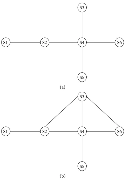
number of the edges that actually exist based on train service plan of the 𝑖th node. In other words, the CC represents the influence of the stations in the network. For example, as shown in Figure 4(b), node S4 has actual connections with nodes S2, S3, S5, and S6. In this case, 𝑘𝑖= 4 which consists of 6 edges. i.e.,

S4-S2, S4-S3, S4-S5, S4-S6, S2-S3, and S3-S6. The maximum number of edges of node S4 is 4 × (4 + 1)/2 = 10. However, only 6 connections actually exist in the network and other 4 edges are not actually existing. In other words, these 4 edges indicate that the connections can be created by using other actual connections, for example, node S4 has not an actual link with node S1 but can use the path S2-S1 to create an edge such as S4-S2-S1. Therefore, by using Equation (5), the CC of S4 is

𝑐6= 2 × 6/4(4 + 1) = 0.6. The CC represents the influence of

the stations in the network, but it has some problems by using the CC in the ranking importance of stations; for example, in some cases, if some of the nodes have same connections in the network, these nodes will have a same value of the CC. This will be demonstrated in the section of case study.

3.5. Comprehensive Factor (CF). In this study, an important factor of CF is introduced in order to integrate degree centrality (5)

𝑐𝑖=_𝑘 2𝑚𝑖

𝑖(𝑘𝑖+ 1),

where 𝑠𝑖 is the SC of a node 𝑣𝑖, and 𝑤𝑖,𝑗 is the weight of the edge between node 𝑣𝑖 and 𝑣𝑗. The weight 𝑤𝑖,𝑗 of an edge between

nodes 𝑣𝑖 and 𝑣𝑗 in the TFN is the number of trains that do stop at the 𝑖th and 𝑗th stations. The SC of a node also describes the service capability of a specific station, which represents the convenience of the passengers from this station to other sta-tions in the network without any change of the train; in other words, trains can reach more stations from the 𝑖th station.

3.3. Betweenness Centrality (BC). The BC as defined in the complex network principles [5] describes the influence of a node in the network; in this case, it is a station in the RPN. In this study, the BC relates to the shortest paths from one node to the other one, i.e., from one station to other station. For every pair of nodes, i.e., between two stations in a network, at least there is one shortest path either it has the minimum number of the edges or it has the minimum value of the weights of the edges. A path is defined as from a node 𝑣𝑗 (i.e., Station 𝑗)

to a node 𝑣𝑘 (i.e., Station 𝑘), which indicates a path passing

between two stations in the network based on train service plan [4, 9]. For example, there are 15 shortest paths between any two nodes in the network as shown in Figure 4(a). Among all the 15 shortest paths, 9 paths pass through node S2 including S1-S2, S1-S2-S4, S1-S2-S4-S3, S1-S2-S4-S5, S1-S2-S4-S6, S2-S4, S2-S4-S3, S2-S4-S5, and S2-S4-S6. But 6 paths that are S3-S4, S3-S4-S5, S3-S4-S6, S5-S4, S6-S4, and S5-S4-S6 do not include the node S2. Therefore, the BC of the node S2 is 9/15 = 0.6.

Assume BC 𝑏𝑖 of a node 𝑣𝑖 in the network without the weight of the edge, which can be calculated by:

where 𝑔𝑗,𝑘 is the number of shortest paths with the minimum

number of the edges from a node 𝑣𝑗 to a node 𝑣𝑘, and 𝑔𝑗,𝑘(𝑖) is

the number of shortest paths with the minimum number of the edges, which pass through the node 𝑣𝑖 from a node 𝑣𝑗 to a node 𝑣𝑘.

Similarly, the BC 𝑏𝑤

𝑖 of a node 𝑣𝑖 with the weight of the edge

is defined as capacity BC, which can be calculated by

where 𝑔𝑤

𝑗,𝑘 is the number of shortest paths with the minimum

sum value of the weights of the edges from a node 𝑣𝑗 to a node 𝑣𝑘, and 𝑔𝑤𝑗,𝑘(𝑖) is the number of shortest paths with the

mini-mum sum value of the weights of the edges, in which trains pass through the node 𝑣𝑖 from a node 𝑣𝑗 to a node 𝑣𝑘. The BC reflects the influence of the nodes throughout the network. A node that has a high impact on network efficiency is called as an influential node. For example, the node S2 in Figure 4(a) is such a node because 9 out of 15 short paths go through this node. Therefore, on the basis of the BC analysis, influential nodes can be obtained in different perspectives of connectivity and transportation capacity.

3.4. Clustering Coefficient (CC). The CC represents a node that links with a certain node, and whether those nodes have also (3)

𝑏𝑖=

∑𝑗 ̸=𝑘𝑔𝑗,𝑘(𝑖)

∑𝑗 ̸=𝑘𝑔𝑗,𝑘 ,

(4)

𝑏𝑤

𝑖 = ∑𝑗 ̸=𝑘𝑔 𝑤 𝑗,𝑘(𝑖)

∑𝑗 ̸=𝑘𝑔𝑤𝑗,𝑘 ,

S3

S4 S6

S2 S1

S5

(a)

S3

S4 S6

S2 S1

S5

(b)

5. Case Study

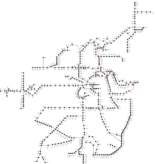
5.1. Background. This section presents a case study on network efficiency analysis for a high-speed rail network to demonstrate the application of the proposed methodology for railway network efficiency analysis. The data and information have been collected from the railway industry for one-day train operation, which indicates that in a total of 2487 trains were operated in such a high-speed rail network. Figure 5 shows the established RPN with 485 nodes (i.e., stations in the network). Based on train service plan on the day, the TFN has also been established with the same number of nodes as the RPN has, i.e., 485 nodes, and the number of edges is analysed as described in Section 2.2; in this case, there are 68198 edges which make up the TFN is more complex than the RPN. Since a large amount of data and information in the network has to be analysed, the new methodology described above has been converted into computer code.

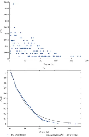
5.2. Degree Centrality (DC) Calculation. As stated in Section  3.1, the distribution of DC can be calculated by Equation (1), for convenience, it has been converted into exponential distribution by

Figure 6(a) shows the results of distribution of DC, and the results of exponential distribution of DC are shown in Figure 6(b). As can be seen that only 11 stations that it is about 2.26% of a total number of stations in the network have a value of DC more than 150. But most of those stations are identified as the hub stations such as Nos. 8, 10, 38, and 48 in Figure 5.

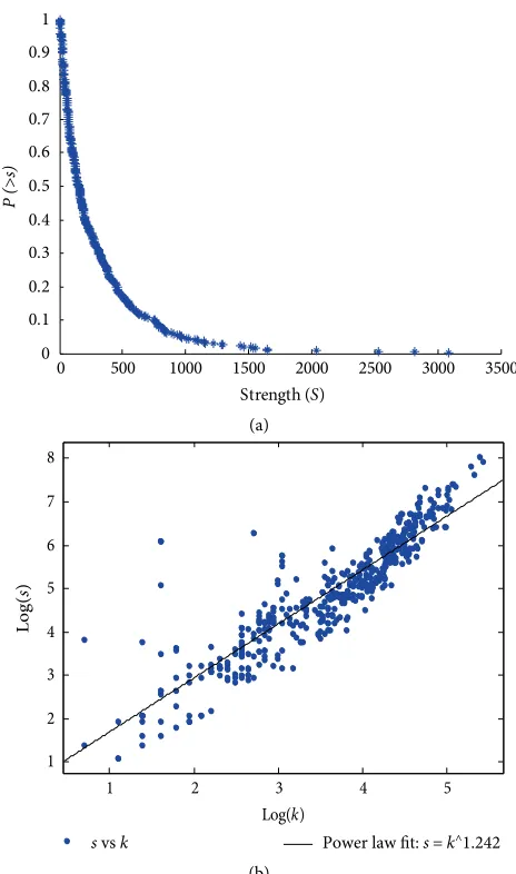
5.3. Strength Centrality (SC) Calculation. The distribution of SC is shown in Figure 7(a), which can be calculated by Equation (2). The results show that only 12 stations (about 4.53%) of total number of stations in the network have a value more than 1000 of SC, and 377 stations (about 77.73%) of total number of stations in the network have a value less than 400 of SC, which indicates that the distribution of SC of the stations in the TFN is extremely deviated, which represents that only a few stations having high service capacity in the network. In other words, it would be more convenient for the passengers to travel from these high service capacity stations than others. Comparing distributions of DC with SC are shown in Figure 7(b), which has been converted by using power law

where 𝑠 can be obtained by Equation (1), and k can be calcu-lated by Equation (2). Equation (11) demonstrates if the con-nectivity of a station in the current transportation operation strategy is 𝑘, the ability to serve the passengers is 𝑘1.242_{. As can}

be seen in Figure 7(b), the SC is increased faster than the DC, in other words, the transportation capacity of a station is grow-ing faster than the growth of connectivity.

5.4. Betweenness Centrality (BC) Calculation. The distributions of BC 𝑏𝑖 and 𝑏𝑖𝑤 (i.e., with/without the weight of an edge) in the

(10)

𝑃(> 𝑠) = 1.09𝑒−0.02_.

(11)

𝑠 ∝ 𝑘1.242_,

(DC), strength centrality (SC), betweenness centrality (BC 𝑏𝑖

and 𝑏𝑤

𝑖 ) and Clustering Coefficient (CC) in a unique manner

for network identification analysis in the TFN. DC, SC, BC (𝑏𝑖

and 𝑏𝑤

𝑖) and CC can be normalized by

Then, the CF 𝐶𝑖 of a node 𝑣𝑖 can be calculated by

where α is the number 1, 2, 3, 4, and 5, i.e., 1 denotes DC, 2 is SC, 3 is BC 𝑏𝑖, 4 is BC 𝑏𝑖𝑤, and 5 is CC, 𝑧𝑖𝛼 represents the values of DC, SC, BC (𝑏𝑖 and 𝑏𝑖𝑤), and CC of a node 𝑣𝑖, 𝑧

min

𝛼 is the

minimum value of DC, SC, BC (𝑏𝑖 and 𝑏𝑖𝑤), and CC of the nodes

in the TFN, 𝑧max

𝛼 is the maximum value of DC, SC, BC (𝑏𝑖 and 𝑏𝑤

𝑖 ) and CC of the nodes in TFN, 𝑧𝛼𝑖 is normalized value of the node 𝑣𝑖, 𝜆𝛼 is the weight of the 𝛼, which shows the impact of

different 𝛼 in the CF. The selection of 𝜆𝛼 depends on the eval-uation purposes such as the connectivity and transportation capacity. For example, if DC, SC, BC (𝑏𝑖 and 𝑏𝑖𝑤), and CC of

the nodes are taken as equally important, then 𝜆 can be chosen as 1/5. If transportation capacity in the TFN is more important than connectivity in the RFN, then 𝜆 can be 2/5. Expert judge-ment and engineering judgejudge-ment such as the Delphi method [30] can be used in the selection of 𝜆𝛼.

4. A New Methodology for Network Efficiency

Analysis

Network reliability can be obtained by the analysis of the char-acteristics of the network under selective and random station failure modes in the railway network [29]. Selective failure mode will enable network analysts to select stations in the railway network based on the current status of the network and their experience to analyse the network reliability, while random failure mode will enable network analysts to assess network efficiency by selecting stations randomly in the rail-way network. The network efficiency 𝐸 and relative network efficiency 𝑅 are given below to evaluate the reliability of the TFN, which are derived by

where 𝑁 is the total number of nodes in the network after a number of station failures, and 𝑑𝑖,𝑗 denotes the number of

edges in the shortest path between nodes 𝑣𝑖 and 𝑣𝑗, which rep-resents the distance between nodes 𝑣𝑖 and 𝑣𝑗 (if 𝑣𝑖 is not

con-nected with 𝑣𝑗, then 𝑑𝑖,𝑗= +∞, and 𝐸 = 0), and 𝐸 is the

network efficiency after the failures of selected stations, and

𝐸0 is the initial network efficiency, 𝑖 and 𝑗 denote two different

nodes.

(6)

𝑍𝛼

𝑖 = 𝑍

𝛼 𝑖 − 𝑍min𝛼

𝑍max

𝛼 − 𝑍

min

𝛼 , 𝛼 = 1, 2, 3, 4, 5.

(7)

𝐶𝑖= ∑ 𝜆𝛼𝑍 𝛼

𝑖, 𝛼 = 1, 2, 3, 4, 5,

(8)

𝐸 = _{𝑁(𝑁 − 1)}2 ∑𝑁

𝑖≥𝑗

1 𝑑𝑖,𝑗,

(9)

5.5. Clustering Coefficient Calculation. The CC can be calculated by using Equation (5). Figure 9(a) shows the distribution of the CC in the cast study. The average of CC in the TFN is 0.697, which demonstrates high aggregation characteristics of the TFN, i.e., stations within the railway network are closely connected. The relationship between the CC and DC of each node is shown in Figure 9(b). As can be seen from Figure 9(b) that, obviously, a node with high CC has a low value of DC. In other words, the TFN are given in Table 1 and shown in Figure 8, which can

be calculated by Equations (3) and (4). Most of the stations have a small value of probability of 𝑏𝑖 and 𝑏𝑖𝑤. Value ranges of

BC 𝑏𝑖 and BC 𝑏𝑖𝑤 in Table 1 are presented as percentage. Only 5

stations have a large value of 𝑏𝑖, which shows that 1.8% of total

stations in the railway network with a value between 0.05730 and 0.06548. In other words, these 5 stations are important and contribute significantly to the efficiency of the TFN.

390 391 392 393 60 185 42 256 33 54 186 103 203 20 181 180 116 4 61 245 49 6 207 146 30 257 117 191 140 148 77 189 165 149 169 124 195 16 15 101 199 201 266 ₂₁₅ 107 200 18 35 81

84 253 273 152 19 209 52 91 151 150 194 198 156 252 85 231 7 36 28 8 261 32 21 259 272 51 9 37 262 182 53 230 63 3 71 227 264 234 128 270 132 229 224 48 221 27 250 130 29 268 72 73 109 24 173 242 153 57 67 79 154 69 56 5 403 404 405 406 407 408 409 410 411 412 414 413 415 416 417 418 419 210 216 263 55 127 131 161 119 80 222 236 147 134 9

188 ₁₉₆ 125

197

436 438 439

440 441

442

437

21311

106 2 135 168 445

446 443

444

447 448 449 450 451 170 10 187 94 87 204 62 86 247 248 38 34 78 13 10089 239 114 208 113 39 5 157 433 434435 95 129 45 65 202 220 99 237 265 96 70 88 68 112 183 136 43 258 58 2 297 296 295 292 190 178 31 26 25 206

41 267 271₄₀ 176 138 162 118 192 211 235 177 108 246 174 160 14 17 74 193 219 44 137 126 172 115 47 46 64 144 158 98 164 92 255 254 251 260 159 22 23 145 105 123 166 76 82 83 179 380 457 456 454 453 452 133 ₃₈₉ 388 387 386 385 384 383 382 381 379 378 377 323 322 321 320 319 318 317 316 315 314 313 333 348 332 342 343 344 345 ₃₄₆ 347 305 312 311 307308 310 306 309 331 330 329 328 327 326 325 324 301 300 299 298 ₃₀₂ 304 59 334335 ₃₃₆ 337 ₃₃₈ 339 ₃₄₀ 341 370 369 368 367 366 365 364 358 357 356 355 ₃₅₃

352 351 354 350 349 363 362 361 360 359 293 294 131 31 284 285 286 287 288 289 290 291 283 282 281 280 279 278 277 218 217 75 141 276 1 244 275 110 142 41 274 455 401 139 402 420 421 422 423 102 167 232

66 473 474 475 476 477 478 479 480 481 482

483 484 485

4 104 163 205 226 233

12 184 225 175 122 212 223

111

143 238 228 50 97 ₂₁₄ 243 240 171 249 90 121 93 241 269 155 44 424 425 426 427 428 429 430 431 466 461 460 459 458

472 471 470 467 468 469 462

463 464 465

371 372 373 374 375 376 303

399 398 397 396 395 394

120

400

432

the values of the DC of the stations. In comparison of the rankings based on values of the CF of the stations with the rankings based on values of the DC, SC, BC (𝑏𝑖, BC 𝑏𝑖𝑤), CBC

and CC of stations, as can be seen that rankings of stations are different. The reason is that the evaluations of DC, SC, BC (𝑏𝑖 and 𝑏𝑖𝑤) and CC have different focuses as discussed in

Sections 3.1–3.5. However, the CF addresses all of issues that focuses on DC, SC, BC 𝑏𝑖, BC 𝑏𝑖𝑤 and CC have; in other words,

CF not only takes the railway network physical topology, but also the operation strategies into consideration such as train running routes, original stations and destination stations, stop-schedules, and service frequencies. Therefore, by using lower value of the DC the station has, the greater value of the

CC that the station has.

5.6. Comprehensive Factor. The CF can be calculated by Equations (6) and (7). Table 2 shows the results and station important rankings of top 20 stations based on their values of the CF, and these stations are also presented in Figure 5 denoted by red spots. Table 2 also shows rankings based on values of DC, SC, TBC, CBC, and CC, respectively. For example, in the column of station (DC), the rankings are based on the values of the DC of the stations, which station identity numbers are given that can be found in Figure 5 and

0 50 100 150 200 250

0 0.005 0.01 0.015 0.02 0.025 0.03 0.035 0.04 0.045

Degree (k)

P (k)

(a)

0 50 100 150 200

0 0.1 0.2 0.3 0.4 0.5 0.6 0.7 0.8 0.9 1

Degree (k)

P (>k)

DC Distribution Exponential fit: P(k)=1.09*_e^_(-0.02)

(b)

edges of the TFN are changed, and application of a single DC or SC or BC 𝑏𝑖, or BC 𝑏𝑤

𝑖or CC cannot provide reliable

results; CF takes all the factors that DC, SC, BC 𝑏𝑖, BC 𝑏𝑖𝑤

, and CC used in the consideration; therefore, by using CF, more reliable results can be obtained. The results of this case study have been further confirmed by the industry from their observation in the railway network [5].

Additionally, based on the results produced by the evalu-ation using CF, as can be seen that most of nodes (i.e., stevalu-ations) with the high values of CF are in the central and eastern regions in the railway network as shown in Figure 5. This is particularly true because this is also confirmed that these areas have a high economic development with high populations and high level of demand of transportation. However, it should be noted that it is not all of these top 20 stations are in the areas with high economic development and high populations. For example, although station Nos. 11, 40, 41, 58, 96, and 174 have higher values of CF, these stations only have one rail line pass through as shown in Figure 5. In order words, these stations (i.e., nodes) have lower physical connectivity in the RPN but have a higher transportation capacity because the frequency of trains using these stations is high. In other words, more trains are scheduled to use these stations. Another interesting finding is that the stations Nos. 259 and 266 in the capital city, are ranked in the places of 17th _{and 14}th_{, and this is because}

there are four stations in the capital city to decentralize trans-port pressure. Other issues should be noted as stated in Section 3.4, in some cases, the application of the CC in the ranking importance of stations is not effective. In this case, as can be seen from Table 2, the top 20 stations have a same value of the CC because these stations have a same number of con-nections with other stations in the network.

5.7. Network Efficiency Analysis. In this case, the average network distance of RPN and TFN can be obtained as 30.84 and 2.89 by analysing the network. In other words, the average network distance 30.84 in the RPN represents that a passenger travels from an original station to a destination CF in the assessment railway network efficiency, more reliable

results can be obtained. This can be demonstrated that, for example, in an emergency, a train may be delayed or cancelled; in this case, the RPN is not changed, but the weights and

0 500 1000 1500 2000 2500 3000 3500

0 0.1 0.2 0.3 0.4 0.5 0.6 0.7 0.8 0.9 1

Strength (S)

P (>s)

(a)

1 2 3 4 5

1 2 3 4 5 6 7 8

Log(k)

Log(

s

)

s vs k Power law fit: s = k^_1.242

(b)

Figure 7: (a) Distribution of SC and (b) DC versus SC.

Table 1: Distributions of BC 𝑏𝑖 and 𝑏𝑖𝑤. Value range of BC 𝑏𝑖

and BC 𝑏𝑤

𝑖 Probability of BC 𝑏𝑖 Probability of BC 𝑏

𝑤 𝑖

0.00000–0.00005 0.168498 0.161172

0.00005–0.00030 0.131868 0.146520

0.00030–0.00100 0.194139 0.201465

0.00100–0.00307 0.197802 0.201465

0.00307–0.00501 0.124542 0.10989

0.00501–0.00603 0.036630 0.032967

0.00603–0.01037 0.058608 0.058608

0.01037–0.02206 0.040293 0.040293

0.02206–0.05730 0.029304 0.029304

0.05730–0.06548 0.018315 0.018315

bi biw

0 50 100 150 200 250 300

Node 0.07

0.06

0.05

0.04

0.03

0.02

0.01

0

BC

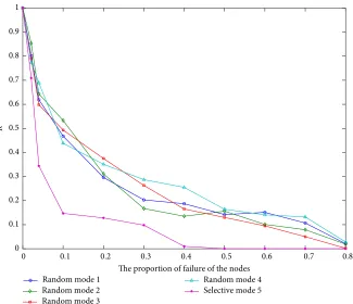
TFN is higher than the RPN, in other words, this represents physical connectivity of the railway network in this case is not very dense, but it has a high service capacity and convenient transportation services. The relative network efficiency 𝑅 can be calculated by Equation (9). Figure 10 shows distributions of 𝑅 under different station failure modes based on selective and random failure modes. Selective mode 5 shows the percentage of failures of top 20 stations, which presents that relative network efficiency is declined sharply until 10% of top 20 station failure. When 40% of top 20 station failures, efficiency 𝑅 of the railway network is near the zero. Random station that at an average the passenger needs to pass through

about 31 (30.84 ≈ 31) stations, and the average network distance 2.89 in the TFN represents the average number of trains that a passenger changes trains during the travel in the railway network. In this case, the passenger needs to change 2 (2.89 − 1 = 1.89 ≈ 2) trains at an average during the travel from an original station to a destination station in the railway network. The network efficiency can be calculated by Equation (8) as described in Section 4, which shows that the network efficiency of the TFN is 2.10, and the RPN is 0.06. This demonstrates that the network efficiency of the

0 0.1 0.2 0.3 0.4 0.5 0.6 0.7 0.8 0.9 1 0.1

0.2 0.3 0.4 0.5 0.6 0.7 0.8 0.9 1

Clustering coefficient (CE)

P

(>CE)

(a)

0 50 100 150 200 250

0 0.1 0.2 0.3 0.4 0.5 0.6 0.7 0.8 0.9 1

Degree k

Clustering coefficient (CE)

(b)

Figure 9: (a) Distributions of CC and (b) CC versus DC.

Table 2: Ranking of top 20 stations. Rank Station (DC) Station (SC) Station (BC 𝑏𝑖) Station (BC 𝑏𝑤

𝑖) Station (CF) Station (CC)

1 8 (229.0) 8 (3088.0) 5 (0.065478) 29 (0.065478) 8 (2.909347)

88, 89, 90, 197, 209, 215, 217, 219, 234, 235, 246, 250, 257,

258, 259, 260, 261, 266, 267, 272 have a same value of the CC 2 10 (221.0) 10 (2813.0) 69 (0.065424) 48 (0.065423) 10 (2.856245)

which will not only balance the distribution of the key stations in the network and relieves the transportation pressure but also help to improve the network efficiency.

The combination of RPN and TFN indicates that some stations are located in the same city, for instance, 4 stations in the capital city. Some hub links between these stations should be allocated in the future, which can not only to improve the physical connectivity of the network and transportation ser-vices but also improve the efficiency of the whole network in different failure modes.

5.7.2. Railway Transportation Operation. According to the efficiency analysis of the railway network, once the key stations are failed or lost service capacity, the connectivity and efficiency of the overall network would drop down rapidly. To ensure the railway network to provide service, it is recommended to establish operation and maintenance strategies to protect these key stations in the railway network in case of emergency, for example, accidents and incidents, and extreme weather. Furthermore, service capacity can be improved by optimising operation scheme with the constraints of the existing RPN. As described in Section 3.1, the higher k is in the network, the higher service capacity of the network can provide. Therefore, a better operation scheme can also increase efficiency of the railway network.

6. Conclusions

The paper presented a new method to analyse the efficiency of the railway network by identifying the key stations based models 1, 2, 3, and 4 show efficiency 𝑅 under randomly

selected percentage of the station failures in the network. The following assumptions are made to implement the selection of random modes [4, 9]:

(i) All stations in the network have an equal opportunity to be selected.

(ii) Each station may be/may not be selected at every time or not.

(iii) Selections of stations start from 10% of station fail-ures to 80% of station failfail-ures in every random mode. As can be seen from Figure 10, when 80% of stations in the network fail to provide service in random modes, the network efficiency 𝑅 is near the zero. Therefore, in compar-ison results of selective mode with random modes, the iden-tified top 20 stations as key stations in the network have high impacts on the network efficiency, which require more attention in operation and further development in the rail-way network. Based on the results produced by the railrail-way network efficiency analysis, recommendations for improve-ment and optimisation of a railway network can be made, which should address two aspects in the planning and operation.

5.7.1. Railway Network Infrastructure Planning. The network efficiency should be considered in the future railway infrastructure planning by taking the economic and demographic factors into consideration. In this case, some of stations with a high CF in the network only have one railway line passing through, and these stations should consider a new rail line to be constructed,

0 0.1 0.2 0.3 0.4 0.5 0.6 0.7 0.8 The proportion of failure of the nodes

0 0.1 0.2 0.3 0.4 0.5 0.6 0.7 0.8 0.9 1

R

Random mode 1 Random mode 2 Random mode 3

Random mode 4 Selective mode 5

[2] M. An, W. Lin, and A. Stirling, “Fuzzy-reasoning-based approach to qualitative railway Risk assessment,” Proceedings of the Institution of Mechanical Engineers, Part F: Journal of Rail and Rapid Transit, vol. 220, no. 2, pp. 153–167, 2006.

[3] M. An, S. Huang, and C. J. Baker, “Railway risk assessment – the FRA and FAHP approaches: a case study of shunting at Waterloo depot,” Proceedings of the Institution of Mechanical Engineers, Part F: Journal of Rail and Rapid Transit, vol. 221, pp. 1–19, 2007. [4] X. Meng, W. Xiang, and L. Wang, “Controllability of train

service network,” Mathematical Problems in Engineering, vol. 2015, Article ID 631492, 2015.

[5] M. Ouyang, L. Zhao, L. Hong, and Z. Pan, “Comparisons of complex network based models and real train flow model to analyse Chinese railway vulnerability,” Reliability Engineering and System Safety, vol. 123, pp. 38–46, 2014.

[6] A. Nagurney and Q. Qiang, “A network efficiency measure with application to critical infrastructure networks,” Global Optimization, vol. 2008, no. 40, pp. 261–275, 2008.

[7] L. Wang, M. An, Y. Zhang, and K. Rana, “Railway network reliability analysis based on key station identification using complex network theory: a real-world case study of high-speed rail network,” in International Research Conference 2017 (IRC 2017): Shaping Tomorrow’s Built Environment, 11–12 October 2017, University of Salford, UK, pp. 395–408, 2017.

[8] L. Li, L. Jia, Y. Wang, and J. Li, “Reliability evaluation for complex system based on connectivity reliability of network model,” in Proceedings of 2015 International Conference on Logistics, Informatics and Service Sciences (LISS), IEEE, Barcelona, Spain, pp. 1–5, 27–29 July, 2015.

[9] M. Saleh, Y. Esa, and A. Mohamed, “Applications of complex network analysis in electric power systems,” Energies, vol. 11, no. 6, pp. 1–16, 2018.

[10] H. Zenil, N. A. Kiani, and J. Tegnér, “Methods of information theory and algorithmic complexity for network biology,” 2014, http://arxiv.org/abs/1401.3604.

[11] L. C. Yin, H. Kretschmer, R. A. Hanneman, and Z. Y. Liu, “Connection and stratification in research collaboration: an analysis of the COLLNET network,” Information Processing & Management, vol. 42, no. 6, pp. 1599–1613, 2006.

[12] M. A. Koseoglu, “Mapping the institutional collaboration network of strategic management research: 1980–2014,”

Scientometrics, vol. 109, no. 1, pp. 203–226, 2016.

[13] D. P. Chassin and C. Posse, “Evaluating North American electric grid reliability using the Barabási-Albert network model,”

Physica A: Statistical Mechanics and its Applications, vol. 355, no. 2–4, pp. 667–677, 2005.

[14] X. L. An, L. Zhang, Y. Z. Li, and J. G. Zhang, “Synchronization analysis of complex networks with multi-weights and its application in public traffic network,” Physica A: Statistical Mechanics and its Applications, vol. 412, pp. 149–156, 2014. [15] A. Vázquez, R. Pastor-Satorras, and A. Vespignani, “Large-scale

topological and dynamical properties of the internet,” Physical Review E: Statistical, Nonlinear, and Soft Matter Physics, vol. 65, no. 6, Article ID 066130, 2002.

[16] P. Dey, R. Mehra, F. Kazi, S. Wagh, and N. M. Singh, “Impact of topology on the propagation of cascading failure in power grid,”

IEEE Transactions on Smart Grid, vol. 7, no. 4, pp. 1970–1978, 2016.

[17] E. Zio and G. Sansavini, “Modeling interdependent network systems for identifying cascade-safe operating margins,” IEEE Transactions on Reliability, vol. 60, no. 1, pp. 94–101, 2011. on the two network models of RPN and TFN. Both physical

network topology and dynamic operation strategies are con-sidered in this method. Considering the key stations, railway network efficiency can be analysed under selective and ran-dom failure modes. A real case study on a high-speed railway network is presented to demonstrate the application of the proposed method. In this case, the key stations can be iden-tified based on the CF in which connectivity, transportation capacity and local influence are taken into consideration. The results show that the identified key stations in the railway network play an important role in improving the overall rail-way network efficiency, which provide useful information to railway designers, engineers, operators and maintainers to operate and maintain railway network effectively and efficiently.

As stated above, the proposed new method considers phys-ical network topology and dynamic operation strategies in the railway network efficiency analysis process. As suggestions, the following aspects in future work may need to be considered to obtain information on availability and stability of the rail-way network. Research should address (1) application of the proposed method by taking railway transportation organiza-tion strategy into physical network consideraorganiza-tion to establish a vehicle flow network for railway transportation organization availability analysis, (2) methods to maintain key stations within a railway network as normal service in an emergency because of an accident or incident occurred, and (3) methods to assess the existing networks by increasing number of new stations while improving efficiency of the railway network.

Data Availability

The readers can find the data used to support the findings of this study are included within the article.

Conflicts of Interest

The authors declare that they have no conflicts of interest.

Acknowledgments

This work describes herein is part of research projects funded by National Key Research and Development Programme of China on “Safety and Security Technology of High-speed Railway System (Grant No. 2016YFB1200401), National Natural Science Foundation of China on “Research on Theory and Methodology of Train Operation Adjustment in Urban Regional Railway Network under Special Conditions (Grant No. 71701010), and Highways England on “New Methodology for Maintenance Decision Making of Structures (Grant No. 546037-PMRB13). Their support is gratefully acknowledged.

References

[18] S. V. Buldyrev, R. Parshani, G. Paul, H. E. Stanley, and S. Havlin, “Catastrophic cascade of failures in interdependent networks,”

Nature, vol. 464, no. 7291, pp. 1025–1028, 2010.

[19] H. P. Ren, J. Song, R. Yang, M. S. Baptista, and C. Grebogi, “Cascade failure analysis of power grid using new load distribution law and node removal rule,” Physica A: Statistical Mechanics and its Applications, vol. 442, pp. 239–251, 2016. [20] J. Yan, H. He, and Y. Sun, “Integrated security analysis on

cascading failure in complex networks,” IEEE Transactions on Information Forensics and Security, vol. 9, no. 3, pp. 451–463, 2014.

[21] S. Dunn and S. Wilkinson, “Hazard tolerance of spatially distributed complex networks,” Reliability Engineering and System Safety, vol. 157, pp. 1–12, 2017.

[22] X. Xu, J. Hu, F. Liu, and L. Liu, “Scaling and correlations in three bus-transport networks of China,” Physica A: Statistical Mechanics and its Applications, vol. 374, no. 1, pp. 441–448, 2007.

[23] S. Porta, P. Crucitti, and V. Latora, “The network analysis of urban streets: a dual approach,” Physica A: Statistical Mechanics and its Applications, vol. 369, no. 2, pp. 853–866, 2006. [24] G. Bagler, “Analysis of the airport network of India as a complex

weighted network,” Physica A: Statistical Mechanics and its Applications, vol. 387, no. 12, pp. 2972–2980, 2008.

[25] L. Dall’Asta, A. Barrat, M. Barthélemy, and A. Vespignani, “Vulnerability of weighted networks,” Journal of Statistical Mechanics: Theory and Experiment, vol. 2006, no. 4, 2006. [26] R. Guidotti, P. Gardoni, and Y. Chen, “Network reliability

analysis with link and nodal weights and auxiliary nodes,”

Structural Safety, vol. 65, pp. 12–26, 2017.

[27] Y. Qian, B. Wang, Y. Xue, J. Zeng, and N. Wang, “A simulation of the cascading failure of a complex network model by considering the characteristics of road traffic conditions,”

Nonlinear Dynamics, vol. 80, no. 1–2, pp. 413–420, 2015. [28] S. Chen, X. Zou, Q. Xu, and H. Lv, “Invulnerability optimization

of Chinese railway traffic network for suppressing cascading failure,” Journal of Information and Computational Science, vol. 11, no. 5, pp. 1501–1509, 2014.

[29] S. Lin, L. Jia, Y. Wang, Y. Qin, and M. Li, “Reliability study of bogie system of high-speed train based on complex networks theory,” in Proceedings of the 2015 International Conference on Electrical and Information Technologies for Rail Transportation, Springer Berlin Heidelberg, pp. 117–124, 2016.

International Journal of

Aerospace

Engineering

www.hindawi.com Volume 2018

Robotics

Hindawi

www.hindawi.com Volume 2018

Hindawi

www.hindawi.com Volume 2018

Active and Passive Electronic Components

VLSI Design

Hindawi

www.hindawi.com Volume 2018

Hindawi

www.hindawi.com Volume 2018 Shock and Vibration Hindawi

www.hindawi.com Volume 2018

Civil Engineering

Acoustics and VibrationAdvances in

Hindawi

www.hindawi.com Volume 2018

Hindawi

www.hindawi.com Volume 2018 Electrical and Computer Engineering

Journal of

Advances in OptoElectronics

Hindawi

www.hindawi.com Volume 2018

Hindawi Publishing Corporation

http://www.hindawi.com Volume 2013 Hindawi

www.hindawi.com

The Scientific

World Journal

Volume 2018

Control Science and Engineering Journal of

Hindawi

www.hindawi.com Volume 2018

Hindawi www.hindawi.com

Journal of

Engineering

Sensors

Hindawi

www.hindawi.com Volume 2018 Hindawi

www.hindawi.com Volume 2018

Modelling & Simulation in Engineering

Hindawi

www.hindawi.com Volume 2018

Hindawi

www.hindawi.com Volume 2018

Chemical Engineering

International Journal of Antennas and Propagation International Journal of

Hindawi

www.hindawi.com Volume 2018 Hindawi

www.hindawi.com Volume 2018 Navigation and Observation International Journal of

Hindawi

www.hindawi.com Volume 2018

Multimedia