Construction and Characterization of 3D Receptive Fields in Mouse Primary Auditory Cortex

2018 International Conference on Applied Mechanics, Mathematics, Modeling and Simulation (AMMMS 2018) ISBN: 978-1-60595-589-6

Construction and Characterization of 3D Receptive Fields in Mouse

Primary Auditory Cortex

Farhad Ahmad Qureshi

and Jun YAN

Department of Physiology and Pharmacology, University of Calgary, Cumming School of Medicine 3330 Hospital Drive NW, Calgary Alberta Canada, T2N 4N1

*Corresponding author

Keywords: 3D rendering, Image processing, Brain signal processing, VTK, Auditory cortex, Hearing research, Spectro-temporal receptive fields, Frequency tuning.

Abstract. Neurons in the central auditory system exhibit non-linear responses to acoustic stimulation. Such nonlinearities are usually illustrated by frequency tuning curves, spectro-temporal response areas and dynamic ranges. None of these methods provide a complete representation of the neural responses in frequency, intensity and timing domains. A novel tool is developed that creates neural response representation across all three domains showing the pattern of excitation as well as inhibition. The primary auditory cortex is selected as the region to create this three dimensional representation as it is a core area of the auditory information processing. The 3D receptive field consists of three visualizations: volume rendering, surface rendering and 2D slicing. All the three visualizations enable the presentation and description of the neural responses to sound in a comprehensive fashion. The 3D receptive field will provide more detailed information when comparing one brain region with the other and can also be used to improve the efficiency of different hearing related devices such as cochlear implants.

Introduction

Our brain is indeed the most complex organ in the body. Not only does it control our emotions and movements but also it takes care of processing the sensory information necessary for us to survive in the world. The brain is made up of some hundreds of billions of building blocks or neurons [13]. A neuron sends and receives binary information as action potentials or spikes. Although there are many types of neurons in the brain, their structure is basically the same [11]. Different regions of the brain have different functions of neurons. For example, neurons in the visual system process visual information from the eyes whereas neurons in the auditory system process auditory information from the ear. How auditory neurons process sound information, or how neurons respond to acoustic signals, is the motivation of this study despite being a hundred-year-old question.

The auditory system is a highly dynamic system. Neurons in the central auditory system often exhibit non-linear responses to both simple and complex sound stimulation [6]. Such nonlinearity can be well illustrated by receptive fields (RFs) [12] that encompass the response properties of auditory neurons to acoustic signals. The RF is commonly presented in three different ways, i.e., frequency response curve, frequency threshold tunings and spectro-temporal response area. The frequency response curve is the frequency tuning exhibiting only spectral information encoded by auditory neurons [17]. The frequency threshold tuning demonstrates the level dynamics of frequency tunings [19]. The spectro-temporal response area is also called the spectro-temporal receptive field (STRF) [1, 2], showing the temporal pattern of frequency tuning at given sound intensity. Since sound is a series of events in time, the temporal pattern of neural response can be more informative to auditory neurophysiologists. The STRF has been an important tool in studying neural processing of sound information in brain, such as the auditory cortex (AC) [3, 7, 9, 10, 15, 22].

RFs bear auditory information in all three domains, i.e., the frequency, intensity and timing domains. In this study, the concept of STRF is further extended and STRF at each sound intensity level is combined to create a 3D version of the STRF which will be referred to as iSTRF. This novel tool comprehensively demonstrates neural firings at frequency, intensity and timing domains in one visualization or illustrative object.

Experimental Techniques

A total of 29 female C57 mice, of age 7-9 weeks and average weight 19.6-24.6 g were used to record bioelectrical signals from the primary auditory cortex (AI). The design of experimental procedures conformed to the ‘Guidelines to the Care and Use of Experimental Animals’ set up by the Canadian Council on Animal Care and was implemented after approval from University of Calgary’s Animal Care Committee under protocol number: AC14-0215. The mouse was anesthetized by a mixture of ketamine (120 mg/kg, i.p., Bimeda-MTC Animal Health Inc.) and xylazine (5mg/kg, i.p., Bimeda-MTC Animal Health Inc. Canada). All surgical procedures were performed under anesthesia. A custom made soundproof chamber was used for performing all experiments. The mouse was kept in this chamber for providing acoustic stimulation and recording biolectrical signals. A multi-frequency gamma tone stimulus design was implemented such that tones of 50-ms duration logarithmically spaced between 5 kHz and 40 kHz at a ratio of 1.0443 [21] were presented to the animal. The choice of logarithmic spacing in tone frequencies was because of the logarithmic distribution of frequencies at the basilar membrane and also due to the logarithmic nature of auditory filters[18]. Tungsten electrodes having tip impedance of ~2 MΩ were used for recording extracellular bioelectrical signals.

Construction and Characterization of iSTRF

The recorded responses were loaded on Matlab (The Mathworks, Inc., Natick, Massachusetts, United States) and processed to extract spike timings for each frequency in the multi frequency stimulus. First, 2D STRFs were created by determining spike timings in milliseconds for each of 50 frequencies delivered. Since 50 sound frequencies were used to stimulate the animal and if e.g. 26 sound intensity levels were used, then for 200 ms duration time window one 2D matrix had dimensions of 50 x 200. A total of 26 such matrices (for each intensity level) were then created and stacked to form a 3D matrix with dimensions 50x200x26. This was our 3D matrix for the iSTRF that is also called the volume of data [5]. The 3D matrix was imported in Python (ver. 2.7.13) for characterization, quantification and creating 3D visualizations of the neural response.

Characterization of Neural Response

Characterization of the iSTRF was performed in line with the conventional 2D characterization techniques such as on the basis of characteristic frequency (CF) which is the frequency showing maximum response at the lowest sound intensity level, best frequency (BF) which is the frequency showing maximum response among all intensity levels, minimum threshold (MT) which is the minimum sound intensity required to evoke a response, latency which is the minimum time required to elicit a neural response and bandwidth (BW), which is the range of frequencies to which a neuron is sensitive to at particular intensity level. The iSTRF is able to perform all the 2D characterization that is necessary to quantify the neural response. Most of the characterization on the neural response is performed after selecting the data at a certain percent of the maximum response in order to get rid of the unnecessary background noise which is also called thresholding. This percentage value is selected based on when a clear receptive field is defined after applying threshold [14].

Quantification

morphological closing is performed by first applying dilation and then erosion. This creates a binary image segmented at half of the maximum response. The thresholded volume is then iteratted to calculate the BW: the first and the last frequencies where response occurs is detected across all slices (for overall BW) and across a particular intensity level (for BW at a particular intensity level) and then the bandwidth of the response BWis calculated by:

BW = F2 – F1 (1) In a similar manner latency of the response was also calculated by detecting the first time bin where a thresholded value existed across all slices. The smallest slice number where a thresholded value was detected represented the MT of the response. Similarly, CF was calculated by determining the maximum spike number at MT and BF was the frequency at which maximum spike number existed across all slices.

Results

3D Visualizations

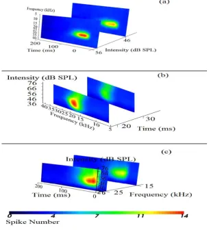
Three type of visualizations were created in Python using the Visualization toolkit (VTK ver. 6.3.0): 2D slicing, volume rendering and surface rendering. For all visualizations, color contours were used to indicate the strength (spike number) of neural response. The regions of high activity (excitation) were represented by warm colors (red to yellow) while those of low or suppressed activity (inhibition) by cool colors (green to blue). The time axis represented the time after tone onset in milisecods (ms), the frequency axis represented the frequencies used to stimulate neurons in kilo Hertz (kHz) and the intensity axis represented the sound intensities in decibel sound pressure level (dB SPL) used for each frequency. The following three visualzaitions were created in Python using VTK:

Figure 1. 2D Slicing: (a) The conventional STRF with level precision. Slices showed at only 56 and 46 dB SPL for simplicity (b) Classical intensity tuning with temporal precision (slices at 20 and 30 ms.) (c) Responses

Two-Dimension Slicing. The 2D slicing feature enables response slicing across different domains. Referring to (Fig. 1a) 2D slicing across intensity domain provides the conventional STRF at each intensity level, (Fig. 1b) shows slicing across time domain enabling the view of FTC at any time instant. The (Fig.1c) show slicing across the frequency domain enabling response to be seen as a function of intensity and time. The following VTK classes were used: vtkColorTransferFunction,

vtkImageResliceMapper, vtk.vtkImageProperty, vtkImageSlice, vtkAxisActor and vtkScalarBarActor.

The neuron in this example had a BF of 19.2 kHz. Slicing across the time axis shows the frequency-amplitude representation of the response (Fig.1b). Similar to STRF this could also be dragged at each time instant and FTCs at each millisecond of the response can be visualized, or in other words the FTCs can be seen with temporal precision (slices at only 20 and 30 ms in Fig. 1b). The shape represented a slant lower FTC. The slicing across frequency axis in (Fig.1c) represents the amplitude-time distribution of the responses with spectral precision enabling the visualization at each stimulus frequency. Since the responses were confined from 15 - 25 kHz, we only included slices within this range. The short latency of the neuron is also visible from this view. The neuron fired maximally within a range of 20 – 56 dB SPL.

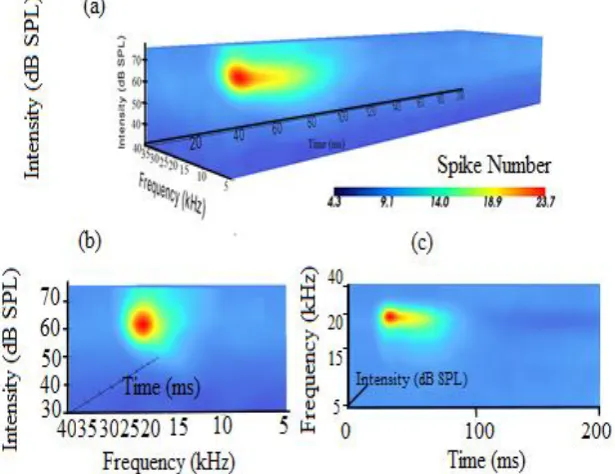
Figure 2. Volume rendering: (a) A complete representation of auditory response across intensity, frequency and time domains. The software enables rotating the volume to view it from different directions. (b) iSTRF view across

frequency amplitude domain. (c) iSTRF view across frequency time domain.

Volume Rendering. A complete representation of the neural response is created using the volume rendering technique. Volume rendering is an extenstion of the 2D STRF with the inclusion of sound intensity information. This representation of the response comprehensively characterized neural response properties such as CF, BF, BW, MT and latency. The VTK classes used for creating this visualization are: vtkImageCast, vtkVolumeRayCastMIPFunction, vtkVolumeRayCastMapper

vtkColorTransferFunction, vtkPiecewiseFunction, vtkVolumeProperty, vtkVolume, vtkAxisActor and

vtkScalarBareActor.

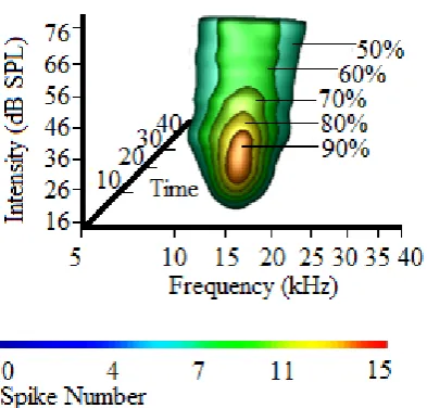
Figure 3. Surface rendering showing surfaces created at 50,60,70,80 and 90% contour levels from the maximum. The surfaces are rendered on top of one another with different opacity levels.

Surface Rendering. Surface rendering is an extension of the 2D contour plot (Fig. 3). Similar to the contouring performed on STRF, a contoured version of the iSTRF was also created using surface rendering. An isosurface plot draws the surface through all points having similar scalar values. This characterizes neural response at different contour levels and shows how the neuron’s best response is shaping towards its characteristic frequency region. The surface resulting from surface rendering would represent the excitatory surface of the iSTRF at different levels from the maximum. It would show the structure and shape of the auditory response across all three domains. This is an interactive way of showing frequency tuning of the neuron illustrating how bandwidth becomes sharper towards the CF region. The VTK classes used for surface rendering are: vtkImageCast,

vtkVolumeRayCastIsosurfaceFunction, vtkVolumeRayCastMapper,

vtkColorTransferFunction,vtkVolumeProperty, vtkVolume, vtkAxisActor and vtkScalarBarActor.

The (Fig. 3) is an example of surface rendering representing excitatory FTC-like iSTRF of the neuron at different levels from the maximum. In this example we rendered surfaces resulting from 50, 60, 70,80 and 90% contour levels on top of one another. This visualization is able to illustrate the BF/MT and latency (if rotated across time domain). The neuron in this example has a U-Shaped FTC with the same CF and BF of 14.1 kHz. This shape also exemplified the majority of our sampled neurons. Similar to the contouring performed on STRF, this visualization could be used for the comparison of the 50% bandwidth of the neuron. The neuron in this example had a bandwidth of 0.74 octaves at 50% contour level (~ 20 dB above threshold). Also, bandwidth at all other contour levels could be extracted.

Discussion

The processing of auditory information from the periphery to the cortex is a transformative process that undergoes numerous enhancements. These transformations are generally studied in two domains, such as the comparison of FTC or STRF of one brain region with the other. A potential application of the iSTRF is to compare different auditory regions in the brain and to examine how different their neural processing is by using more detailed information. The iSTRF would comprehensively define the auditory region under study in one representation. This application can easily extend to the evaluation of hearing deficiencies such as hearing loss. Another application of the iSTRF could be to test the functionality of different hearing devices such as cochlear implants. The iSTRF can provide a response pattern (e.g Fig. 2a ) from a healthy and intact hearing system which could be used to improve the efficiency of cochlear implants and other hearing related devices.

For further work, a best response pattern of the neuron could be extracted using the 3D processing and a sound signal could be designed to stimulate neurons defined by that pattern. This sound signal could form the identity or fingerprint of the particular auditory neuron under study.

Conclusion

The iSTRF serves as a complete package to study auditory neural response properties. The quantification and characterization performed on the iSTRF is in line with the previous techniques. The iSTRF gives a complete description of the auditory neural response in one representation. The visualizations are highly interactive and show more insights into the firing pattern of auditory neurons as compared to the previous techniques.

Acknowledgements

This work is supported by the grants from the Canadian Institutes of Health Research (Grant # 274494), the Natural Sciences and Engineering Research Council of Canada (DG261338- 2009) and the Campbell McLaurin Chair for Hearing Deficiencies at the University of Calgary. The authors declare no competing financial interests.

References

[1] Aertsen AM, Johannesma PI. (1981a) The spectro-temporal receptive field. A functional characteristic of auditory neurons. Biol Cybern. 42(2):133-43.

[2] Aertsen AM, Johannesma PI. (1981b) A comparison of the spectro-temporal sensitivity of auditory neurons to tonal and natural stimuli. Biol Cybern. 42(2):145-56.

[3] Aertsen, A. M. H. J., Olders, J. H. J., & Johannesma, P. I. M. (1981). Spectro-temporal receptive fields of auditory neurons in the grassfrog.Biological cybernetics, 39(3), 195-209.

[4] Barbour, D. L., & Wang, X. (2003). Contrast tuning in auditory cortex. Science, 299(5609), 1073-1075.

[5] Calhoun, P. S., Kuszyk, B. S., Heath, D. G., Carley, J. C., & Fishman, E. K. (1999). Three-dimensional volume rendering of spiral CT data: theory and method. Radiographics, 19(3), 745-764.

[6] Cartwright, J. H., González, D. L., & Piro, O. (2001). Pitch perception: A dynamical-systems perspective. Proceedings of the National Academy of Sciences, 98(9), 4855-4859.

[7] Depireux, D. A., Simon, J. Z., Klein, D. J., & Shamma, S. A. (2001). Spectro-temporal response field characterization with dynamic ripples in ferret primary auditory cortex. Journal of neurophysiology, 85(3), 1220-1234.

[8] Ebert, L. C., Schweitzer, W., Gascho, D., Ruder, T. D., Flach, P. M., Thali, M. J., & Ampanozi, G. (2017). Forensic 3D visualization of CT data using cinematic volume rendering: a preliminary study. American Journal of Roentgenology, 208(2), 233-240.

[10] Gourévitch, B., Noreña, A., Shaw, G., Eggermont, J.J., (2009). Spectro-temporal receptive fields in anesthetized cat primary auditory cortex are context dependent. Cereb. Cortex 19, 1448e1461. [11] Haken, H. (2007). Brain dynamics: an introduction to models and simulations. Springer Science

& Business Media.

[12] Hartline, H. K. (1940). The receptive fields of optic nerve fibers. American Journal of Physiology—Legacy Content, 130(4), 690-699.

[13] Kandel, E. R., Schwartz, J. H., and Jessel, T. M. (2000). Principles of Neural Science.

[14] Liang, F., Bai, L., Tao, H. W., Zhang, L. I., & Xiao, Z. (2014). Thresholding of auditory cortical representation by background noise. Frontiers in neural circuits, 8, 133.

[15] Miller, L. M., Escabí, M. A., Read, H. L., & Schreiner, C. E. (2002). Spectrotemporal receptive fields in the lemniscal auditory thalamus and cortex. Journal of neurophysiology, 87(1), 516-527. [16] Muthusami, P., Shkumat, N., Rea, V., Chiu, A. H., & Shroff, M. (2017). CT reconstruction and MRI fusion of 3D rotational angiography in the evaluation of pediatric cerebrovascular lesions. Neuroradiology, 59(6), 625-633.

[17] Schreiner, C. E., Read, H. L., & Sutter, M. L. (2000). Modular organization of frequency integration in primary auditory cortex. Annual review of neuroscience, 23(1), 501-529.

[18] Sutter, M. L. (2000). Shapes and level tolerances of frequency tuning curves in primary auditory cortex: quantitative measures and population codes. Journal of neurophysiology, 84(2), 1012-1025.

[19] Temchin, A. N., Rich, N. C., & Ruggero, M. A. (2008). Threshold tuning curves of chinchilla auditory-nerve fibers. I. Dependence on characteristic frequency and relation to the magnitudes of cochlear vibrations. Journal of neurophysiology, 100(5), 2889-2898.

[20] Vahlensieck, M., Lang, P., Chan, W. P., Grampp, S., & Genant, H. K. (1992). Three-dimensional reconstruction. European Radiology, 2(6), 503-507.

[21] Valentine, P. A., & Eggermont, J. J. (2004). Stimulus dependence of spectro-temporal receptive fields in cat primary auditory cortex. Hearing research, 196(1), 119-133.