2018 2nd International Conference on Applied Mathematics, Modeling and Simulation (AMMS 2018) ISBN: 978-1-60595-580-3
A Deterministic Global Optimization Method for Solving
Generalized Linear Multiplicative Programming
Problem with Multiplicative Constraints
Bo ZHANG and Yue-lin GAO
*Research Institute of Information and System Computation Science, North Minzu University, Yinchuan, 750021, China
*Corresponding author
Keywords: Global optimization, Linear multiplicative programming, Linear relaxation, Branch and bound.
Abstract. This paper presents a deterministic global optimization algorithm for solving generalized linear multiplicative programming problem with multiplicative constraints (GLMP). By utilizing equivalent transformation and linear relaxation method, a linear relaxation programming (LRP) of equivalent problem (GLMPH) is established. In the algorithm, lower and upper bounds are simultaneously obtained by solving some linear relaxation programming problems (LRP). Global convergence has been proved and results of some sample examples and a small random experiment show that the proposed algorithm is feasible and efficient.
Introduction
The Generalized linear multiplicative programming(GLMP) refers to a type of optimization problems,which contains the sum of the product terms of two real functions in objective or constraint functions,is a special category of multiplicative programming. The plentiful researchers and scholars have attached importance to this topic for many years.In this paper, we consider the following generalized linear multiplicative programming (GLMP):
. |
, , , 2 , 1 , 0 )
( . .
) ( min
(GLM P) s
0
1
1 0 0 0 0
0
b Ax R x X x
N s
f x e d x c x
G t s
f x e d x c x
G
n p
i si
T si si T si s
p
i i
T i i T
i
WherecsiRn,esiRn,i1,2,,ps,s0,1,2,,N ,while the constant terms dsi, fsiare all
arbitrary real numbers, ARmnis a matrix,bRmis a vector,set X is nonempty and bounded.
During the past years, (GLMP) has received significant attention in the literature because there are many practical applications in different fields of research, including multiple-objective decision[1],Robust optimization[2], plant layout design[3], financial optimization[4] and so on. Of course,there are many ways to solve this problem and we can see these methods in articles[5-11].
New Linearization Skill
For each j1,2,n, compute lj minxX xj and uj maxxXxj ,and define the vector l and u as
follows:
nT
n R
l l l
l 1, 2,, ,
n T
n R
u u u
u 1, 2,, ,Obviously,ljxjuj.Then, the hyper-rectangle H
x l x u
u
l, ] |
[ , which can cover the feasible domainFXis obtained.
It is distinct that
( ) ( ) .) (
1 s
T s T s s s s T
s s T p
i si
T si si T si
s x c x d e x f x ce x c f ed x d f
G
s
N s R f R d R e R
c s s s ps
s p s p n s p n
s , , , , 1,2,,
.
In view of x ce x x ecT x
s s T T s s T ) ( )
( , we can easily obtain
. 2 2 ) ( ) ( )
(c e x x c e x x ec x x c e e c x
x T s s T s s T T s s T T s s T T s s T Let 2 T s s T s s s c e e c
Q ,then, nn
s R
Q is a real symmetric matrix.Assume i
min
is the minimum eigenvalue
of the matricesQs,for i1,2,,p.If min 0
s
,lets 0 ;otherwise, let
s
s min ,where 0 then
I
Qss is semi-positive definite.
On the rectangleHk
xRn lk xuk
H| ,for each s,we construct a linear lower function of
) (x Gs on
k H .Because ) ( ) ( ) ( ) ( ) ( ) ( x f d x d e f c x f d x d e f c x e c x x G s s T s T s s s s s s T s T s s s s T s s T s (1)
Where, x x Qs sI x
T
s( ) ( )
is a convex function and ( ) ( )
1 2
n j j x x is a concave function. Then
without any loss of generality, we can reformulate the (GLMP) problem as the following problem
) (GLMPH :
. , , 2 , 1 , 0 ) ( ) ( ) ( ) ( . . ) ( ) ( ) ( ) ( min : 0 0 0 0 0 0 0 0 0 X H x N s x f d x d e f c x x G t s x f d x d e f c x x GGLMPH s s
T s T s s s s s s T T
Suppose k
j
l and k j
u is the j-th indicator of k
l and k
u respectively. We know that, for each
1, 2,j ,n
, the linear equation through the two endpoints on the parabola 2j
x is
2 ) ( : j k j k j j k j k j
j l u x l u x
y
L ,therefore, x2j yj (ljk ukj)xj lkjukj,and then,
( )
( ) ( ) , . ( ) ( 1 12 n k k k T k k
j k j k j j k j k j n
j xj l u x l u l u x l u x H
x
)
(2) According to the convexity of s(x), we can have
) ( ) ( ) ( )
(x x0 x x0 T s x0
s
s
.
On the basis of the sub-differential definition, we know that s(x)s(x), Without loss of generality,
for all the arbitrary real vector k
H
x0 ,so s(x0)s(x0)2(QssI)x0.
This implies that
. , ) ( ) ( 2 )
( 0T s s 0T s s 0 k
s x x Q I xx Q I x xH
(3) Let 2 0 k k k mid u l x
x , thereupon,the lower bound estimation function of (x) and s(x) is
obtained,we construct the following linear function
. , , 2 , 1 , 0 , , ) ( )
(x x x H s N
G k k
s T k s k
. 2 ) ( 2 ) ( ), ( 2 ) ( 2 k k s s T k k k T k s s T s k s k k s s s s s k k s s k s u l I Q u l u l f d u l d e f c u l I Q
Theorem 1 For each s{0,1,2,,m}, let QssI be semi-positive definite. For each s{0,1,2,,N},
the linear function Gks(x) is a lower function of G (x)
k
s on the rectangle
k
H , i.e.G (x) Gks(x)
k
s ,
k
H x
.
Proof From the formula (1),(2) and (3), for each s{0,1,2,,N}, we have
. , ) ( ) ( ) ( ) ( )
( sk k
T k s s s T s T s s s s s
s x x c f ed x d f x x x H
G
Consequently, G (x) Gks(x)
k
s ,
k
H x
,s{0,1,2,,N}. Theorem 2 Let j uj lj,(j1,2,,n),for every
k
H
x ,when j 0,the gap between Gs(x) and )
(x
Gs satisfies Gs(x)Gs(x)0,s{0,1,2,,N}.
Proof For convenience of proving Theorem 2, Let k k k k
u l x
x , mid, , denote x,xmid,l,u at the beginning of
the k-th iteration , respectively .From the formula (1) and (4), we have
. ) ) ( ( ) ( ) ( ) ( ) )( ( ) ( ) ( 2 2 k k s s s k k k k s k mid k s s k k T k k s k mid k s s T k mid k k s k s l u I Q x u l x x x I Q x u l x x x I Q x x x G x G Where(QssI)is the spectral radius of the rectangle QssI, apparently, whenj 0,j1,2,,n,
0
2 2
l
u , Gs(x)Gs(x)0,s{0,1,2,,N}.Hence, the conclusion is established.
Therefore, from the theorem 1, we obtain the linear relaxation programming problem of (GLMPH)
on the rectangle k
H : . , , , 2 , 1 , . . ) ( min : ) ( 0 X H x N s x t s x G LRP k k s k s k k
According to the above, we only need to solve the problem (LRPk), whose optimal value v(LRPk) is
a lower bound of the global optimum value ( k)
GLMPH
v of the problem (GLMPH) on rectangle k
H ,the
optimal value v(LRPk) also is an effective lower bound of the global optimum value v(GLMPk) of
the original problem (GLMP)onHk,i.e. ( k) ( k) ( k)
GLMP v
GLMPH v
LRP
v .
Meanwhile, Theorem 2 ensures that problem (LRPk)can infinitely approximate the primitive
problem, as X →0, this will guarantee the global convergence of the proposed algorithm.
The Subdivision and Reducing of the Rectangle
In this section, the bisection and reducing methods of the rectangle are given. Let Hk lk uk H
] ,
[ is a
rectangle on n
R , and k k
H
x .
The Subdivision OF the Rectangle
The method of the subdivision of the sub-hyper- rectangle is depicted as follows:
Firstly, computing
x l
u xk
j n
j k j k j k
j : 1,2, ,
max
, if 0, Select the longest edge of the
rec-Tangle Hk,i.e.
n j l u l u k j k j k k , , 2 , 1 :
max
,then xk(uk lk)/2;if 0,then finding the first
k j
x arg max,let k
j k
x
x . Secondly, let
k n k j k k j k k l l x l l l
x 1,2,, 1, , 1,, ,
k n k j k k j k k u u x u u u
Through the straight line or plane about the pointxand pointx, the rectangularHkis divided into two sub super rectangular k1 [ k1, k1]
u l
H and k2 [ k2, k2]
u l
H , then the sub-super-rectangular Hk1and
2
k
H are respectively:
]. , [ ] , [ ] , [ ],
, [ ] , [ ] , [
1 1
1 2 1
1
1
1 k
j k j n
j k k k j k j j k k j k j n
j k k k j k j j k
u l u
x u l H
u l x
l u l H
The Reducing of the Rectangle
Based on literature [12], in order to improve the convergence of the algorithm, we present two pruning methods,which can be used to eliminate the region in which the global optimal solution of
)
(GLMP problem does not exist.For any Hk
xRn|lk xuk
H,assume the objective of ( k)
LRP is ,
)
( 1 0 0
0
n
j
k j k
j k
x x
G and the constraints are 1 ik,
n
j j
k
ijx b
a
the current known upper bound of theoptimal value *
0
G of (GLMP) is denoted by UB. For every i1,2,,Nm,s1,2,,n,we must follow the following rules:
Rule 1 Compute k s
and min{ 0 , 0 k}
s k
s k s k
sl u
, if min{ 0 , 0 k}
s k
s k s k
s k
s l u
then Hkis deleted; otherwise, if
0
0
k s
and 0 k,
s k
s k
s u
let
k
s k
s k s k
s u
u min ,
0
; if 0k 0
s
and 0 k,
s k
s k
s l
let
k
s k
s k s k
s l
l max ,
0
.
Rule 2 Compute k is
and min{ , k}
s k is k s k isl a u
a ,if min{ , k}
s k is k s k is k
is a l a u
,then k
H is deleted; otherwise, if
0
k is
a and k
s k is k is a u
,let
k
s k is k is k
s u
a
u min , ;if k 0
is
a and k
s k is k is a l
,let
k
s k is k is k
s l
a l max , .
Where,
, } ,
min{ 0
,
1 0 0
k n
s j j
k j k
j k j k
j k
s UB l u
n s j j
k j k ij k j k ij k
i k
is b 1, min{a l ,a u }
.
Algorithm and its Convergence
Next, a branch and bound reduced algorithm of problem (GLMP) is described.
Suppose when the iteration proceed in step k, the feasible region of the problem (GLMP) is denoted
by F,Hkrepresent the divided rectangle soon, Wrepresent the feasible set at present, the set of
remained the super rectangle after pruning is denoted by T.L is the lower bound of global optimal
value of the problem (GLMP);U said the upper bound of global optimal value of (GLMP).
Step 1 (initializing)
Constructing n-dimensional super-rectangleH[l,u] covering the feasible region F; Solving the
problem ( 0)
LRP , its optimal value and optimal solution is denoted by 0( 0)
0 x
G and x0 respectively.
) (
0 0
k
x G
L is a lower bound of global optimal value of the problem(GLMP);if xLF
,let
Lx W
W ; if W,then let U min
G0(x):xW
,and finding a current optimal solution x argminG0U .Set
0
and let T
H ,k1.Step 2 (termination rule)
If ULor T , then the calculation is stopped, The global optimal solution 0( )
U
x
G of the
output problem(GLMP),Otherwise go to the next step.
Step 3 (selection rule)
The super rectangle k
H , which corresponds to the minimum lower bound L, is selected,in T,
i.e. k L
H
H ;
Step 4 (subdivision rule)
Using the subdivision method of the first part of the third section, then the super rectangle Hkcan
be cut apart into sub-rectangles k1
H and k2
H , and k1 k2
H
Step 5 (reducing technique)
Reducing the sub-rectangles after dividing using the reducing method of the second part of the third
section,for convenience,the new sub-rectangles after reducing are also denoted by ki
H , and
i ,where is the index set of the rectangles after reducing.
Step 6 (upper bounding)
If W, let U,else U min
G0(x):xW
,The current optimal solution is x argminG0U .
Step 7 (pruning rule)
Let TT
Hk Gk xk U xkHk T
, ) ( :
\ 0 .
Step 8 (lower bounding)
If
T ,let LU,else Lmin
G0k(xk):xkHk T
Step 9 Set kk1, go to step 2.
Theorem 3 (a) If the algorithm terminates within finite iterations with an globally optimal solution for (GLMP) be found.
(b) If the algorithm generates an infinite sequence of iterations, then any accumulation point of the sequence {xk}is a global optimal solution of the
) (GLMP .
Proof (a) If the algorithm is finite, assume it stops at the k-th iteration,k ≥1.From the termination
rule of Step 2, we know that UL.Based on the upper bounding technique described in Step 6, it
implies that G0(xk)L,From the Step 4 and Step 6,we also know the globally optimal solution is
U
x ,we known that U G xk G xU L
) ( )
( 0
0 .Hence, Combined these inequalities, we obtained that
) ( )
( )
( 0 0
0
k U
k
x G L x
G x
G , and then the part (a) has been proven.
(b) If the algorithm is infinite, and an infinite feasible solution sequence { k}
x is generated of the
problem (GLMP) by solving the problem (LRPk). According to the Step 6 and Step 8 of the algorithm,
we have
, 2 , 1 ), ( ) ( )
( 0 0
0
G x G x G x k
L k k U k
(5) Because the series
0k( k)
x
G is non-decreasing and bounded, and
0( k)
x
G is non-increasing and
bounded, then the series
0k( k)
xG and
0( k)
x
G are both convergent. Take the limit on the both side of
(5), we have
). ( lim ) ( ) (
lim 0 0 0 k
k U k
k
kG x G x G x (6)
And then lim 0( )
k k
k G x
L , lim 0( ),
k
k G x
U
the formula (6) convert into L G0(x ) limG0(x ) U.
k k
U
Without loss of generality, assume the rectangle sequence
Hk [lk,uk]
satisfy k kH
x and
k k
H H 1
.In our algorithm, the rectangles are divided into two parts of the equal width continuously,
then { }
1
k k
k H x
because of the continuity of function 0( k)
x
G , ( ) lim ( ) ( *),
0 0
0 x G x U G x
G
L k
k
U
So the
sequence of { k}
x whose any accumulation point is a global optimal solution of problem (GLMP).
Numerical Experiments
We coded the algorithms in Matlab 2016a, and ran the tests in a PC with Intel(R) Core(TM) i5-4210M processor of 2.6GHz, 4 GB of RAM memory, under the Win7 operational system .The simplex method is applied to solve the LRPs. Table 1 or 2 shows that our algorithm performs are efficient. In
our experiments, the convergence tolerance is 10-8.
iterations, this indicates that our new relaxation technique can be better applied to some problems where the optimal solution is located in the corner of the feasible region. At here, the notations used in the head line have the following means: Iter: average numbers of iterations in the algorithm; Time: average CPU time in seconds; lam: denote the number of the associated tolerance; p,m and n denote the number of the product term,linear constraints ,variables and the multiplicative constraints, respectively.
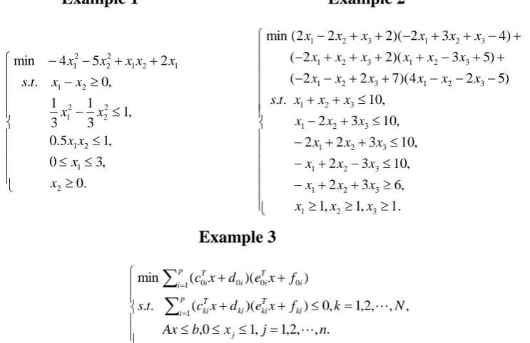
Example 1 Example 2
. 1 , 1 , 1 , 6 3 2 , 10 3 2 , 10 3 2 2 , 10 3 2 , 10 . . ) 5 2 4 )( 7 2 2 ( ) 5 3 )( 2 2 ( ) 4 3 2 )( 2 2 2 ( min . 0 , 3 0 , 1 5 . 0 , 1 3 1 3 1 , 0 . . 2 5 4 min 3 2 1 3 2 1 3 2 1 3 2 1 3 2 1 3 2 1 3 2 1 3 2 1 3 2 1 3 2 1 3 2 1 3 2 1 2 1 2 1 2 2 2 1 2 1 1 2 1 2 2 2 1 x x x x x x x x x x x x x x x x x x t s x x x x x x x x x x x x x x x x x x x x x x x x x x t s x x x x x Example 3
. , , 2 , 1 , 1 0 , , , , 2 , 1 , 0 ) )( ( . . ) )( ( min 11 0 0 0 0
[image:6.595.116.488.171.412.2]n j x b Ax N k f x e d x c t s f x e d x c j p i ki T ki ki T ki p i i T i i T i
Table 1. Results of the numerical contrast experiments 1–2.
E M x* f(x*) Iter Time lam
[image:6.595.87.509.440.545.2]1 Ours [9] [10] (2.0000, 1.0000) (2.0000, 1.0000) (2.0000, 1.0000) −15.000 −15.000 −15.000 20 110 1657 0.4837 57.224 120.58 1e-8 1e-8 1e-6 2 Ours [11] [12] (5.5556,1.7778, 2.6667) (5.5556,1.7778,2.6667) (5.5556,1.7778, 2.6667) -112.754 -112.754 -112.754 49 57 5 1.4302 - 1.1491 1e-8 1e-3 1e-6
Table 2. Numerical results of Example 3.
p m n N Iter Time
5 5 10 5 33.10 2.3154
5 10 10 5 31.61 2.2663
10 20 10 5 44.35 2.3731
10 20 20 5 61.50 3.6550
10 20 10 10 23.15 1.3220
20 20 20 5 94.61 6.8459
20 20 20 10 45.55 4.4356
20 20 30 10 105.73 13.7012
20 20 40 5 381.75 39.9987
elements of fki is pseudo-randomly generated in the range [-1, 0], k{1, 2, , }N . For this problem, we tested twenty different random instances and listed the computational results in Table 2.
As can be seen from Table 2, the size of p, m,n and N have a corresponding effect on them. With the change of p, I and t alter correspondingly when the other three variables are fixed, and there is no rule. If p,m and n are fixed, both t and I decrease with the increase of n. As soon as the p,m and N has been determined,with the increase of N, both t and I are also increasing. When p, n and N remain unchanged, t and I also decrease with the increase of m.
Concluding Remarks
In this study, the performance of the algorithm is different depending on the situation of the four variables. Our algorithm have no requirement for the size of p if the number of m, n and N is determined. Moreover, our algorithm has a wider range of applications than the method for solving a single linear multiplicative programming problem .
Acknowledgement
This research was financially supported by National Natural Science Foundation of China (No. 61561001), National Science and technology leadership project (No. 2015KJ003) ,Postgraduate Innovation Project of North Minzu University (YCX18084) and the Project of First-rate discipline Construction in Ning xia higher Education (NXYLXK2017B09).
References
[1] Keeney RL, Raiffa H. Decisions with multiple objective. Cambridge, MA: Cambridge University Press; 1993.
[2] Mulvey JM, Vanderbei RJ, Zenios SA (1995) Robust optimization of large-scale systems. Oper Res 43:264–81.
[3] Quesada I, Grossmann I E. Alternative Bounding Approximations for the Global Optimization of Various Engineering Design Problems [M]// Global Optimization in Engineering Design.Springer US, 1996:309-331.
[4] C. D. Maranas, I. P. Androulakis, C. A. Floudas, A. J. Berger, and J. M. Mulvey, “Solvinglong-term financial planning problems via global optimization,” Journal of Economic Dynamics and Control, vol. 21, no. 8-9, pp. 1405–1425, 1997.
[5] Fan Q, Wu W, Zurada J M. Convergence of batch gradient learning with smoothing regula- rization and adaptive momentum for neural networks [J]. Springerplus, 2016, 5(1):1-17.
[6] Zhou X G, Cao B Y, Wu K. Global optimization method for linear multiplicative Programming [J]. Acta Mathematicae Applicatae Sinica English, 2015, 31(2):325-334.
[7] Wang C F, Bai Y Q, Shen P P. A practicable branch-and-bound algorithm for globally solving linear multiplicative programming[J]. Optimization, 2017, 66(3):1-9.
[8] Zhao Y, Liu S. An efficient method for generalized linear multiplicative programming problem with multiplicative constraints[J]. SpringerPlus, 2016, 5(1): 1302.
[9] Shen P, Duan Y, Ma Y. A robust solution approach for nonconvex quadratic programs with additional multiplicative constraints [J]. Applied Mathematics & Computation, 2008, 201(1–2): 514-526.
[11] Wang C F, Bai Y Q, Shen P P. A practicable branch-and-bound algorithm for globally solving linear multiplicative programming[J]. Optimization, 2017, 66(3):1-9.