Research on Supplier Credit Evaluation Based on Data Mining

2018 International Conference on Computer, Communications and Mechatronics Engineering (CCME 2018) ISBN: 978-1-60595-611-4

Research on Supplier Credit Evaluation Based on Data Mining

Ping-hua YANG, Cai-xia YANG and Jie HE

School of Computer Engineering, Guangzhou College of South China University of Technology, Guangzhou, Guangdong 510800, China

Keywords: Credit scoring, Data mining, Logistic model, Weights of evidence.

Abstract. Data mining method is used to clean the real data of suppliers on cost link. With its 80% random drawing as a training set, a WOE and logistic regression model is set up to distinguish the integrity supplier on the platform according to the new calculation formula of WOE for indicator variable. And using the rest 20% as test data to calculate the accuracy of this model which is as high as 96.9%. Finally, the credit score card is established according to the linear scaling relation between the WOE value and regression coefficient of each indicator variable, which can calculate supplier credit score and provide decision-making reference for the platform and users when selecting suppliers.

Introduction

Credit is an important foundation of the market economy. Credit evaluation is an important basis for enterprises to select and motivate suppliers, and is the basis for establishing long-term stable cooperative relations. How to accurately portray the credit of suppliers is of great significance to the improvement of cooperation efficiency and the establishment of credit mechanism[1]. At present, there are many methods for suppliers’ credit evaluation, such as gray correlation method[2], analytic hierarchy process [3-4], genetic clustering method[5], principal component analysis method[6], fuzzy comprehensive evaluation method[3,7], neural network[8-9], logistics regression method[10] etc. Among them, the logistics regression method has excellent comprehensive performance in terms of efficacy, practicability and well-posedness[11], and it is widely used in the dual credit evaluation model, but it also has defects. For example, in practical applications, the acquisition quality of real data is required to be high, and it is necessary to assume a linear relationship between the intermediate variable and the independent variable. As the distance between the distribution of dishonest sample and the distribution of honest samples can be described by the weights of evidence (WOE) method in information theory, it can be used to estimate the probability of supplier dishonesty[11]. Replacing the independent variable with the WOE value of the independent variable for Logistic regression can overcome the difficulty of not satisfying the linearity. Therefore, this paper combines the evidence weighting method with the classical Logistic regression method, and applies it to the real data of the first comprehensive data interaction platform in the domestic construction industry, the real data of the cost-effectiveness, and establishes its supplier's binary credit evaluation classification model to distinguish the integrity. This paper also establish a credit scorecard with a non-integrity supplier based on the linear proportional relationship between the WOE value and the regression coefficient of each independent variable, and calculate the specific credit value score of each supplier, which provides qualitative and quantitative dual-level decision-making reference for the platform and users when screening suppliers.

Data Processing and Analysis

Data Preparing

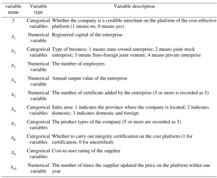
variables, 5 categorical variables). The response variable y is a two-category variable that distinguishes whether the supplier is an honest merchant. The specific variable types and meanings are shown in Table 1.

Table 1. The specific variable types and meanings.

variable name

Variable type

Variable description

y Categorical

variables

Whether the company is a credible merchant on the platform of the cost-effective platform (1 means no, 0 means yes)

1

x Numerical

variable

Registered capital of the enterprise

2

x Categorical

variables

Type of business: 1 means state-owned enterprise; 2 means joint-stock enterprise; 3 means Sino-foreign joint venture; 4 means private enterprise

3

x Numerical

variable

The number of employees

4

x Numerical

variable

Annual output value of the enterprise

5

x Numerical

variable

The number of certificate added by the enterprise (5 or more is recorded as 5)

6

x Categorical

variables

Sales area: 1 indicates the province where the company is located; 2 indicates domestic; 3 indicates domestic and foreign

7

x Categorical

variables

The product types of the company (5 or more are recorded as 5)

8

x Categorical

variables

Whether to carry out integrity certification on the cost platform (1 for certification, 0 for uncertified)

9

x Categorical

variables

Cost-to-user rating of the supplier

10

x Numerical

variable

The number of times the supplier updated the price on the platform within one year

Missing Value Analysis and Processing

The aggr function in the R language can be used to plot the missing values in the data set (Figure 1, red is missing data, blue is normal one).

Figure 1. Data missing situation.

It can be seen that there are only variablesx₁ and x₄missing values in the data set. Calling the

md. pattern function shows that there are 88 missing values in the dataset (50 ofx₁, 38 ofx₄). There

Variable Correlation Analysis

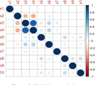
In order to avoid the occurrence of multi-collinearity problems and improve the accuracy of the model, it is necessary to check the correlation between variables before establishing the model. The Corrplot function in the R language is used to plot the correlation between the variables (see Figure 2, the deeper the color, the larger the correlation coefficient, the higher the correlation between the variables).

Figure 2. Variable correlation.

In Figure 2, the intersections of the variables x₃andx₄, as well asx₂ and x₄are darker, showing

a higher correlation between the two sets of variables. Therefore, the variablex₄is removed, and the remaining variables are tested for correlation. The function chart. Correlation is called to display the correlation between the variables in the form of correlation coefficients (see Figure 3).

Figure 3. Variable correlation coefficient graph.

As can be seen in Figure 3, the most relevant set of variables isx3andx6, the correlation coefficient is 0.28, while the correlation coefficient between the other variables is smaller.

Modeling Data Set Segmentation

80% of the 3795 raw data sets from which the variablex₄was removed were randomly selected as the training set, and 20% were used as test sets to establish the model and the test model, respectively.

Supplier Credit Evaluation Model

Establishment of Classical Logistic Regression Model

1

y is recorded as pP y( 1|X) , then the probability that y0 is 1p. The ratio

1

p p

 is the ratio of the odds of the event, recorded asodds. When taking the natural logarithm of odds,

( ) ln( )

Logit p  odds。 can be got. When p(0,1), odds(0,) Logit p( )  ( , ). Establish

a linear regression model Logit p( ) with independent variables X (x x x₁, ₂, ₃,...,x_n), which is

the logistic regression model: g X( )Logit p( )₀_{1 1}x ₂x₂,...,_nx_n.

The regression coefficients of the variables in the model can be obtained by the maximum likelihood estimation, and the AIC value is 339.08. However, the pvalues of the three variables and the three variables were greater than 0.05 and failed to pass the test. Therefore, the three variablesx₁,x₃and x₇were eliminated and the remaining six variables were re-transformed by Logistic regression. The six variables passed the test, and the new model has an AIC value of 334.41, which is smaller than before, indicating that the new model works better.

WOE-based Logistic Regression Model

In the classical logistic regression model, it is assumed that the intermediate variable Logit p( )has

a linear relationship with the independent variableX (x x x₁, ₂, ₃,...,xn), which is not necessarily met in practice. To this end, imitating the formula (7) in [11], the WOE defining the selected

variablex is as follows: WOE( ) ln[( ( 1)) / ( ( 0))]

( 1) ( 0)

n y n y x

m y m y

 



  Among them, n( ) indicates the number of each category in the training sample, m( ) indicates the number of each category in the total sample. That is, the WOE value is the difference between the logarithm of the non-integrity and integrity supplier in the training sample and the logarithm of the non-integrity and integrity supplier ratio in the total sample. It reflects the extent to which this variable affects the supplier's classification results. An increase in the WOE value of the selected variable implies a decrease in the probability of dishonesty. Using the monotonous WOE value as a new independent variable into the Logistic regression model can overcome the difficulty that the intermediate variable Logit p( )

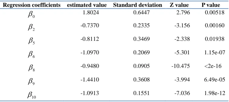
and the original data may be nonlinear, and the regression coefficients are shown in Table 2. At this time, the AIC value is 288.06.

Table 2. Regression coefficient based on WOE value modeling.

Regression coefficients estimated value Standard deviation Z value P value

0

 1.8024 0.6447 2.796 0.00518

2

 -0.7370 0.2335 -3.156 0.00160

5

 -0.8112 0.3469 -2.338 0.01938

6

 -1.0970 0.2069 -5.301 1.15e-07

8

 -0.9480 0.0905 -10.475 <2e-16

9

 -1.4410 0.3608 -3.994 6.49e-05

10

 -1.0913 0.1551 -7.036 1.98e-12

Model Evaluation

value is compared to 0.5 using the if else function, and the output value is converted to 0 and 1 types. The confusion matrix that finally obtains the output predicted value and the true value is shown in Table 3.

Table 3. Confusion matrix.

classification y0

y=0

1

y total

y=0 692 10 702

y=1 14 52 66

total 706 62 768

From the above table, the accuracy of each category of the model can be calculated asy0: 692

98%

706 ;y1: 52

83.8%

62 . The recall rates for each category are y0: 692

98.6% 702 ;

1

y : 52 78.8%

66  . The total accuracy of the model is

692 52

96.9% 768

 _

. It can be seen that the

model has a strong predictive ability.

Credit Score

Establishment of Credit Scorecard

The two-category Logistic regression model established above can distinguish honest and untrustworthy merchants, but cannot judge whoever has higher credit in honest merchants. So the score corresponding to each variable can be obtained according to the linear proportional relationship between the WOE value and the regression coefficient of each variable. The specific calculation formula is: multiply the regression coefficient of the variable coe i( )by the WOE value of the variable, multiply by the set scale factork, and finally add the offsete, that is,

WOE ( )

score coe i  k e (1) When the odds ratioodds15 :1, the corresponding score is set 600, and if the score is 10 higher,

the odds ratio is doubled. Which is 600 ln15 610 ln 30

k e

k e

  



 _{  }

 , it can be solved that

14.4269, 560.9311

k e

From this, the base score for the merchant credit can be calculated as:k coe (1)+e 593

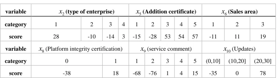
Then, according to formula (1), the binning range of each variable is scored, and the final scorecard is shown in Table 4.

Table 4. Credit scorecard.

variable x₂(type of enterprise) x₅(Addition certificate) x₆(Sales area)

category 1 2 3 4 1 2 3 4 5 1 2 3

score 28 -10 -14 3 -15 -28 53 54 57 -11 11 19

variable x₈(Platform integrity certification) x₉(service comment) x₁₀(Updates)

category 0 1 1 2 3 4 5 (0,10] (10,20] (20,30]

score -38 18 -68 -76 1 4 15 -35 0 78

The final credit score of the merchant is calculated as the base score plus the score corresponding to each part of the variable. Based on this scorecard, you can calculate:

Minimum credit score = 593-14-28-11-38-76-35=391

Scoring Case

Assuming that the data of a supplier of the platform is as shown in Table 5, the credit value of the supplier is divided into 593+3-15-11-38+4-35=501. It can be seen that the credit value of the supplier is relatively general.

Table 5. Variable value and score of a supplier.

variable x₂ x₅ x₆ x₈ x₉ x₁₀

data 4 1 1 0 4 1

Corresponding score 3 -15 -11 -38 4 -35

Conclusion

Based on the registered data of the first comprehensive data interaction platform in the construction industry, the paper uses R language data mining method to establish its supplier credit score model based on WOE and Logistic regression. Tested by the test set, the model can help the platform to screen and screen the network suppliers, and eliminate the bad companies whose credit value is not good, so as to improve the quality of the platform suppliers and provide the best quality choice environment for users.

References

[1] Fang Q. Credit Assessment of Enterprise Suppliers [J]. Logistics Technology, 2009, 28(12):85-86.

[2] Xu J, Qi Zh F. Analysis of Suppliers' Credit Level and Its Grey Correlation Model [J]. Journal of Shanxi Finance and Economics University, 2003, 25(4): 71-74.

[3] Li ZhK, Liu X. Fuzzy Comprehensive Evaluation of Nonferrous Metal Suppliers Based on Green Supply Chain [J]. Statistics and Decision, 2008, (4): 65-66.

[4] Xu Y, Zhang Y. A online credit evaluation method based on AHP and SPA[J]. Communications in Nonlinear Science & Numerical Simulation, 2009, 14(7):3031-3036.

[5] She Ch Y, Liang X J. Algorithm of Genetic Clustering and its Application to Evaluation of Supplier Credit[J]. Journal of China Three Gorges University (Natural Sciences), 2007, 29(3): 242-244.

[6] Li Y, Wang L H. Supplier Credit Evaluation Based on Principal Component Analysis [J]. Commercial Research, 2009, (8): 209-210.

[7] Liu Y D, Gao J. Fuzzy comprehensive evaluation on the supplier credit for manufactory[J].Information Technology, 2008, (4):101-103.

[8] Fu Y G, Zhu J M. Network provider credit evaluation model based on big data [J]. Journal of Central University of Finance and Economics, 2016, (8): 74-83.

[9] Rong F Q, Guo M F. The Study of Credit Evaluation of Suppliers on Cross-border E-commerce Platform Based on Big Data[J]. Statistics & Information Forum, 2018, 33(3): 100-107.

[10] Shi L L, Li Ch Y, J Ch, etc. Minor enterprise credit assessment based on Logistic regression model[J]. Journal of Science of Teachers' College and University, 2018, 38(5):10-17.