2018 IX International Conference on Optimization and Applications (OPTIMA 2018) ISBN: 978-1-60595-587-2
Frontier Visualization for Nonconvex Models with Increasing and
Decreasing Returns to Scale with the Use of Enumeration Methods
Vladimir KRIVONOZHKO
1,2,3,*, Andrey LYCHEV
1, and Nina BLOKHINA
4Federal Research Center “Computer Science and Control”, Russian Academy of Sciences, Vavilov st. 44-2, 119333 Moscow, Russia
National University of Science and Technology MISiS, Leninsky pr. 4, 119049 Moscow, Russia Lomonosov Moscow State University, Faculty of Computational Mathematics and Cybernetics,
GSP-1, Leninskie Gory, 119991 Moscow, Russia
Moscow State University of Civil Engineering, Yaroslavskoye Shosse 26, 129337 Moscow, Russia Corresponding author
Keywords: Free disposal hull, Frontier visualization, Enumeration methods.
Abstract. A lot of scientific literature in the world is devoted to the returns-to-scale (RTS)
evaluation of production units. Kerstens and Vanden Eeckaut were the first who considered the notion and evaluation of RTS for nonconvex Free Disposal Hull (FDH) models. Their methods are based on the comparison of the radial efficiency scores of a production unit in the FDH model and the corresponding non-increasing and non-decreasing RTS reference models. At the same time Cesaroni, Kerstens and Van de Woestyne noted the absence of papers in the world literature devoted to methods of frontier visualization in nonconvex models. In this paper, we developed methods for visualization of production function of nonconvex models and of the corresponding non-increasing and non-decreasing models. Our approach of frontier visualization can be used for decision making based on nonconvex models, it allows us to evaluate RTS for FDH models. Our results are confirmed by computational experiments in applications with real-life data sets.
Introduction
There is a lot of scientific literature in the world devoted to the returns-to-scale (RTS) eval- uation of production units. Data Envelopment Analysis (DEA) models and Free Disposal Hull (FDH) models appeared almost simultaneously in papers [1, 3, 4], respectively, for performance management in complex systems. In DEA models, the production possibility set is a convex set. For this reason, solution methods and software have been widely used for modeling and computa- tions of various indicators of unit’s behavior, including such an important indicator as RTS. On the contrary, the production possibility set of FDH models is a non-convex set, for this reason, the development of these models was refrained. Apparently, Kerstens and Vanden Eeckaut [7] were the first to propose a subtle approach for estimating RTS of production units in FDH models. Their approach is based on the comparison of the input radial efficiency of a unit in the FDH model and the corresponding constant, non-increasing and non-decreasing RTS reference technologies. Such an approach requires solving nonlinear mixed integer optimization problems. In [17], it was proved that these problems can be rewritten as mixed integer linear problems, at the same time the size of such problems increases significantly, what complicates the solution process by these
1 2 3 4
methods. Soleimani-damaneh et al. [19] proposed enumeration algorithm for estimating RTS in FDH models. Leleu [13, 14] suggested a linear programming approach to the same problem. At the same time, the author noted that the proposed linear programming problems do not have any computational advantages over the nonlinear problems, although the former might be easier to program in real-life applications. There have been three papers [19, 20, 21] that simplify the computations needed to implement the method of Kerstens and Vanden Eeckaut [7] to estimate RTS. Podinovski [16] is the first to indicate that the method of Kerstens and Vanden Eeckaut for estimating global returns to scale for nonconvex technologies is incomplete. Moreover, it was shown in [18] that one must distinguish the fourth type of global sub-constant RTS in addition to the three traditional cases (constant, decreasing and increasing returns to scale). Some works are devoted to visualization of Pareto sets in general optimization problems, see, for example, [15].
In this paper, we develop an approach for visualization of FDH frontier with increasing and decreasing returns to scale. Our approach allows us to evaluate returns to scale for FDH models, which requires fewer computations than existing methods.
This paper is structured as follows. Section 2 provides some basic definitions of the convex and less widely applied nonconvex technologies. Section 3 presents two algorithms of frontier visualization for non-convex models with variable, increasing and decreasing returns to scale with the use of enumeration methods. Then follows Section 4 with some computational results. Section 5 concludes.
Preliminaries
Consider a set of n observation of actual production units (Xj, Yj), j = 1, . . . , n, where the vector of outputs Yj = (y1j, . . . , yrj)>0, j = 1, . . . , n is produced from the vector of inputs Xj = (x1j, . . . , xmj) > 0, j = 1, . . . , n. The traditional FDH technology described in [4] is written as follows:
TFDH =
(X, Y)
n
X
j=1
Xjλj ≤X, n
X
j=1
Yjλj ≥Y, n
X
j=1
λj = 1, λj ∈ {0,1}, j = 1, . . . , n
, (1)
where λj,j = 1, . . . , n are integer variables taking on values 0 or 1.
In addition, we consider the constant, non-increasing, non-decreasing returns-to-scale reference technologies associated with the technology TFDH. They are written as follows.
TCRS=
(X, Y)(X, Y) = δ(X0, Y0), (X0, Y0)∈TFDH, δ≥0 ,
TNIRS =
(X, Y)(X, Y) = δ(X0, Y0), (X0, Y0)∈TFDH,0≤δ ≤1 ,
TNDRS=
(X, Y)(X, Y) = δ(X0, Y0), (X0, Y0)∈TFDH, δ≥1 .
(2)
In order to evaluate RTS in FDH technology the reference technology methods require the evaluation of the input or output radial efficiency scores of a given unit (Xo, Yo) in technologyTFDH
and/or in some of three technologies (2). For the sake of being definite, we limit our investigation to the case of input radial efficiency.
The input radial efficiency score Ei
FDH(Xo, Yo) in technologyTFDH can be evaluated by solving
the next mixed integer linear problem:
EFDHi = minθ
subject to n
X
j=1
Xjλj ≤θXo,
n
X
j=1
Yjλj ≥Yo,
n
X
j=1
λj = 1,
λj ∈ {0,1}, j = 1, . . . , n,
(3)
The evaluation of the input radial efficiency of unit (Xo, Yo) in any of the three associated technologies (2) requires more computational effort. In the paper [7], the following general model of the mixed integer nonlinear problems was developed for this purpose:
θo = minθ
subject to n
X
j=1
Xjλj ≤θXo,
n
X
j=1
Yjλj ≥Yo,
λj =δwj,
wj ∈ {0,1}, j = 1, . . . , n,
δ∈Γ, n
X
j=1
wj = 1,
(4)
where the set Γ is defined different by depending on the associated technology, in which the evaluation takes place. Actually, for the CRS, NIRS and NDRS technologies, we use
ΓCRS=
δδ ≥0 ,
ΓNIRS =
δ0≤δ≤1 ,
ΓNDRS =
δδ ≥1 .
(5)
Let Ei
CRS(Xo, Yo), ENIRSi (Xo, Yo) and ENDRSi (Xo, Yo) be the input radial efficiency scores of unit (Xo, Yo) in the reference technologies, in other words, equal to the optimal value θo of prob-lem (4) with the appropriately specified set Γ.
Next, we consider the notion of global RTS (GRS) in the case of FDH technology.
Definition 1 (Banker [2]). Unit (Xo, Yo) is at the most productive scale size (MPSS) if for all units (ϕXo, ψYo)∈TFDH, where ϕ, ψ >0, the ratioψ/ϕ ≤1.
problem:
M∗ = maxψ/ϕ
(ϕXo, ψYo)∈TFDH,
ϕ >0, ψ >0.
(6)
According to Definition 1, unit (Xo, Yo) is at MPSS if and only if M∗ = 1.
Definition 2. Unit (ϕ∗Xo, ψ∗Yo)∈ TFDH is called a scale reference unit (SRU) of unit (Xo, Yo) if ϕ=ϕ∗,ψ =ψ∗ is an optimal solution to problem (6), that is ψ∗/ϕ∗ =M∗.
It is worthy of note that unit (Xo, Yo) may have more than one SRU.
Theorem 1 (Podinovski [16]).Assume that unit (Xo, Yo) is efficient in technology TFDH and is
not at MPSS. Let (ϕXo, ψYo)∈TFDH be its SRU. Then either both ϕand ψ are greater than 1 or
both are smaller than 1.
It follows from this theorem, that we can classify the SRUs of the efficient unit (Xo, Yo) into those smaller (ϕ < 1 andψ <1) and those larger (ϕ >1 and ψ >1) than unit (Xo, Yo).
The definition below categorizes all efficient units into the four mutually exclusive types of global returns to scale (GRS) [16, 18].
Definition 3. Suppose that unit (Xo, Yo) is efficient in technology TFDH. Then unit (Xo, Yo) displays
1. global constant RTS (G-CRS) if unit (Xo, Yo) is at MPSS,
2. global decreasing RTS (G-DRS) if all its SRUs are smaller than unit (Xo, Yo), 3. global increasing RTS (G-IRS) if all its SRUs are larger than unit (Xo, Yo),
4. global sub-constant RTS (G-SCRS) if some its SRUs are smaller, and some are larger than unit (Xo, Yo), but unit (Xo, Yo) itself is not at MPSS.
The following theorem [16] presents us a practical tool for the GRS characterization of efficient units in the FDH model. It is based on the evaluation of input efficiency of unit (Xo, Yo) in FDH model and its NIRS and NDRS reference technologies.
Theorem 2 (Podinovski [16]). Assume that unit (Xo, Yo) is efficient in technology TFDH, then it
displays
1. G-CRS if and only if Ei
NDRS(Xo, Yo) = ENIRSi (Xo, Yo) = EFDHi (Xo, Yo); 2. G-DRS if and only ifENDRSi (Xo, Yo)< ENIRSi (Xo, Yo)≤EFDHi (Xo, Yo); 3. G-IRS if and only ifEi
NIRS(Xo, Yo)< ENDRSi (Xo, Yo)≤EFDHi (Xo, Yo); 4. G-SCRS if and only ifEi
NDRS(Xo, Yo) =ENIRSi (Xo, Yo)< EFDHi (Xo, Yo).
As it was remarked above, evaluating input radial efficiency of unit (Xo, Yo) in FDH model requires solving a mixed integer linear problem. On the other hand, evaluating its efficiency in the NIRS and NDRS technologies is the more complicated problem and requires solving mixed integer nonlinear problems.
Below we develop algorithms that allow us to construct sections on the frontier of the FDH model by two-dimensional planes, which allows us to identify the GRS type of an efficient unit (Xo, Yo) without computing its efficiency scores in reference technologies.
Algorithms for Construction of Efficient Frontier for NIRS and NDRS Technologies
In papers [9, 10], frontier visualization methods were proposed for FDH model based on enu-meration and optimization algorithms. In this section, two methods are developed for construction of efficient frontier for NIRS and NDRS models. This approach allows us to evaluate returns to scale in the FDH model without additional solution of two non-linear mixed integer optimization problems for NIRS and NDRS reference technologies.
Consider any unit (Xo, Yo) ∈ TFDH and any two nonzero vectors (directions) d1, d2 ∈ Em+r,
such that d1 is not parallel to d2. Define two-dimensional plane in the spaceEm+r as
Pl(Xo, Yo, d1, d2) = (Xo, Yo) +αd1+βd2, (7)
where α and β are scalar parameters. The above plane passes through the point (Xo, Yo) and is spanned by the vectors d1 and d2.
Denote WEffPTFDH the weakly (Pareto) efficient frontier of model FDH. Define the intersection
of this frontier with the two-dimensional plane (7) as follows:
Sec(Xo, Yo) =
(X, Y)(X, Y)∈Pl(Xo, Yo, d1, d2)∩WEffP TFDH . (8)
Following papers [9, 12], and by taking different directions d1 andd2, one can construct various
sections of the weakly efficient frontier WEffPTFDH [11]. For our purpose (construction of sections
of the frontier for NIRS and NDRS technologies) we should choose directionsd1 = (Xo,0)∈Em+r and d2 = (0, Yo)∈ Em+r. Introducing parameters ϕ= 1 +α and ψ = 1 +β, we observe that the plane (7) consists of all points that can be written in the form (X, Y) = (ϕXo, ψYo). According to [12], we call such section Sec(Xo, Yo) generalized production function. The corresponding sec-tions Sec(Xo, Yo) of the NIRS and NDRS technologies can be used to evaluate RTS of the FDH model at every point of the FDH section without additional solutions of nonlinear mixed integer optimization problems.
Figure 1 illustrates the work of Algorithm 1. It starts with vertexesZl = (zαl, z β
l ),l= 1, . . . , L, generated by one of the algorithms described in [9, 10]. Next, Algorithm 1 finds k0, the index of
maximal peak of the unit that exhibits maximal production scale size. In this case, k0 = 9, hence
pointP1 =Z9is one with a most productive scale size. Then, define a regionD1 where Algorithm 1
finds next points P2 and P20 of the two-dimensional section for NIRS technology. Iterations are
repeated till the last point is found, in our case point (vertex) P4.
Proposition 1. Algorithm 1 constructs the generalized production function for NIRS technology for a given unit in a finite number of steps.
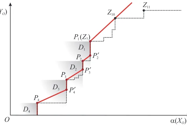
Figure 2 explains the main principle of Algorithm 2. As distinct from the previous algorithm, Algorithm 2 finds at first an index of minimal peak among points that exhibit maximal productive scale size. According to Fig. 2, this is point P1(Z7). Then the region D1 is determined, where
points P2 and P20 are found, and iterations are repeated. Hence, the algorithm moves from right
to the left till the last point is found, in our case, this is pointP4.
Algorithm 1. Construction of production function for NIRS technology
Input: Zl = (zlα, zlβ), l = 1, . . . , L, are vertexes of production function of unit (Xo, Yo) in FDH technology
Output: S, a production function of unit (Xo, Yo) in NIRS
technol-ogy.
1: P0←
pα 0, p
β 0
= (0,0), the first point of the section.
2: D0 ← {1, . . . , L}, the index set of the section in FDH model, it contains all vertexes of the
two-dimensional section at the beginning.
3: R0← j
zjβ
zα j ≥ z β l zα l
, l∈D0
, index set of points with maximal productive scale size.
4: k0←arg max j∈R0
zα
j , the index of maximal peak of the unit that exhibits maximal production scale
size.
5: P1←Zk0, the second point of the NIRS production function.
6: S←
P0, P1
, the first segment of the NIRS section. 7: i←1, initialize counter.
8: whileDi←
lzlα> pαi, z
β l > p
β
i, l∈Di−1 6=∅do
9: Ri ←
j
zjβ
zα j ≥ z β l zα l
, l∈Di
, the index set of points with maximal productive scale size, that
are contained in setDi. 10: ki ←arg max
j∈Ri
zαj , the index of maximal peak of unit that exhibits maximal productive scale
size. 11: Pi+1=
pα i+1, p
β i+1
←Zki, the next angular point of a new section.
12: Pi0+1← pαi+1 p β i pβi+1, p
β i
!
, a new angular point between pointsPi andPi+1.
13: S←S∪
Pi, Pi0+1
∪
P0
i+1, Pi+1
, add two new segments to the constructing section. 14: i←i+ 1, increment counter.
15: end while
16: S←S∪
Pi+γeα
γ≥0 , add a horizontal ray going out from the last point Pi of the section.
17: OutputS.
Computational Experiments
The algorithms described in this paper have been tested with the use of real-life data sets from different areas: Russian banks, Norwegian municipal nursing- and home-care services and Swedish electricity utilities. Original data sets are described in papers [5, 6, 8]. Computational results are illustrated in this paper on the data from Swedish electricity utilities. The number of production units in this dataset is 163. The model has four inputs and four outputs. On the input side we use kilometers of low- and high-voltage power lines and total transformer capacity in kVA as the capital variables. Labor is measured in full-time equivalent employees. As the four outputs, we used the total amount of low- and high-voltage electricity in MWhs delivered to customers and the number of low- and high-voltage customers served. All computational experiments were conducted using a personal computer with Intel Core i3 CPU operating at 3.33 GHz.
In our computational experiments, constructions of stepwise production functions with the help of enumeration algorithm [10] for all units in the FDH model took 0.0893 s. At the same time, constructions of production functions and sections of NIRS model for all units took 0.0965 s. And constructions of production functions and sections of NDRS models together for all units
Figure 1. Construction of production function for NIRS technology
Figure 2. Construction of production function for NDRS technology
required 0.0949 s. These figures showed that the time needed for section constructions for NIRS and NDRS models is negligibly small in comparison with a time required for constructions of production functions for FDH model.
[image:7.612.145.474.368.590.2]en-Algorithm 2. Construction of production function for NDRS technology
Input: Zl= (zαl, zβl),l= 1, . . . , L, are vertexes of production function of unit (Xo, Yo) in FDH model
Output: S, a production function of unit (Xo, Yo) in NDRS
technol-ogy.
1: D0 ← {1, . . . , L}, the index set of the section in FDH model, it contains all vertexes of the
two-dimensional section at the beginning.
2: R0← j
zjβ
zα j ≥ z β l zα l
, l∈D0
, index set of points with maximal productive scale size.
3: k0 ←arg min j∈R0
zα
j , the index of minimal peak of the unit that exhibits maximal productive scale
size.
4: P1←Zk0, the first point of the NDRS section.
5: S←
γP1
γ≥1 , ray is added going out radially from pointP1 to infinity.
6: i←1, initialize counter.
7: whileDi←
lzlα< pαi, z
β l < p
β
i, l∈Di−1 6=∅do
8: Ri ←
j
zjβ
zα j ≥ z β l zα l
, l∈Di
, the index set of points with maximal productive scale size, that
are contained in setDi. 9: ki ← arg min
j∈Ri
zjα , the index of minimal peak of unit that exhibits maximal productive scale
size among units belonging toRi. 10: Pi+1=
pα i+1, p
β i+1
←Zki, the next angular point of a new section.
11: Pi0+1←
pα i, p
β i+1 pα i pα i+1
, a new angular point between pointsPi andPi+1.
12: S←S∪
Pi, Pi0+1 ∪
Pi0+1, Pi+1, add two new segments to the sectionS. Observe, that points of
the section are added in the reverse order, that is pointPi+1is situated on the left from pointPi.
13: i←i+ 1, increment counter.
14: end while
15: S←S∪
Pi−γeβγ≥0 , add to the section a vertical ray starting from last pointPiand going
down. 16: OutputS.
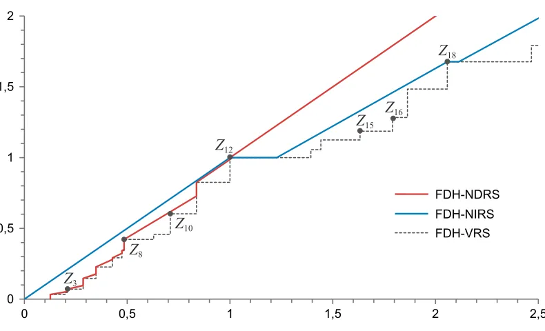
larged part of the section in the vicinity of the origin. The coordinates of this unit in the figure are (1,1). The red line corresponds to NDRS technology, the blue line associates with FDH-NIRS technology, the gray dashed line is the part of the efficient frontier of FDH-VRS model. If lines FDH-NDRS, FDH-NIRS, and FDH-VRS are constructed, then RTS can be easily evaluated at any angular point Z1, . . . , Z15, . . . , Z35 on the curve. Take, for example, point Z8. This point
exhibits increasing RTS, since, according to the results of this paper, this point belongs to the NDRS line. Point Z12 exhibits constant RTS since it belongs to both NDRS and NIRS lines.
Point Z15 is situated very close to the line NIRS, so it exhibits decreasing RTS.
Conclusions
Our work develops an approach for visualization of FDH frontier with increasing and decreasing returns to scale. Our method requires much fewer computations then existing ones. Our computa-tional experiments documented this fact. Next, if the NDRS and NIRS section are constructed, it is not necessary to solve two additional mixed integer optimization problems in order to evaluate
Figure 3. NDRS, NIRS and VRS production functions for unit 290
Figure 4. The enlarged part of Figure 3 around the unit 290
RTS at any point of the curve. It is sufficient to have a look at the figure and to use the results of this paper.
Acknowledgements
References
[1] R. D. Banker, A. Charnes, and W. W. Cooper. Some models for estimating technical and scale inefficiencies in data envelopment analysis. Management Science, 30(9):1078–1092, 1984. [2] Rajiv D. Banker. Estimating most productive scale size using data envelopment analysis.
European Journal of Operational Research, 17(1):35–44, 1984.
[3] A. Charnes, W. W. Cooper, and E. Rhodes. Measuring the efficiency of decision making units.
European Journal of Operational Research, 2(6):429–444, 1978.
[4] D. Deprins, L. Simar, and H. Tulkens. Measuring labor efficiency in post offices. In M. Marc-hand, P. Pestieau, and H. Tulkens, editors,The Performance of Public Enterprises: Concepts and Measurements, chapter 10, pages 243–268. North Holland, Amsterdam, 1984.
[5] Espen Erlandsen and Finn R. Førsund. Efficiency in the provision of municipal nursing- and home-care services: The norwegian experience. In Kevin J. Fox, editor, Efficiency in the Public Sector, chapter 10, pages 273–300. Springer US, Boston, MA, 2002.
[6] F. R. Førsund, L. Hjalmarsson, V. E. Krivonozhko, and O. B. Utkin. Calculation of scale elasticities in DEA models: direct and indirect approaches. Journal of Productivity Analysis, 28(1-2):45–56, 2007.
[7] Kristiaan Kerstens and Philippe Vanden Eeckaut. Estimating returns to scale using non-parametric deterministic technologies: A new method based on goodness-of-fit. European Journal of Operational Research, 113(1):206–214, 1999.
[8] V. E. Krivonozhko, F. R. Førsund, and A. V. Lychev. A note on imposing strong complemen-tary slackness conditions in DEA. European Journal of Operational Research, 220(3):716–721, 2012.
[9] V. E. Krivonozhko and A. V. Lychev. Algorithms for construction of efficient frontier for nonconvex models on the basis of optimization methods. Doklady Mathematics, 96(2):541– 544, 2017.
[10] V. E. Krivonozhko and A. V. Lychev. Frontier visualization for nonconvex models with the use of purposeful enumeration methods. Doklady Mathematics, 96(3):650–653, 2017.
[11] V. E. Krivonozhko, O. B. Utkin, A. V. Volodin, and I. A. Sablin. About the structure of boundary points in DEA. Journal of the Operational Research Society, 56(12):1373–1378, 2005.
[12] V. E. Krivonozhko, O. B. Utkin, A. V. Volodin, I. A. Sablin, and M. V. Patrin. Constructions of economic functions and calculations of marginal rates in DEA using parametric optimization methods. Journal of the Operational Research Society, 55(10):1049–1058, 2004.
[13] H. Leleu. Mixing DEA and FDH models together. Journal of the Operational Research Society, 60(12):1730–1737, 2009.
[14] Herv´e Leleu. A linear programming framework for free disposal hull technologies and cost functions: Primal and dual models. European Journal of Operational Research, 168(2):340– 344, 2006.
[15] Alexander V. Lotov and Kaisa Miettinen. Visualizing the pareto frontier. In J¨urgen Branke, Kalyanmoy Deb, Kaisa Miettinen, and Roman S lowi´nski, editors,Multiobjective Optimization: Interactive and Evolutionary Approaches, pages 213–243. Springer Berlin Heidelberg, Berlin, Heidelberg, 2008.
[16] V. V. Podinovski. Local and global returns to scale in performance measurement. Journal of the Operational Research Society, 55(2):170–178, 2004.
[17] V. V. Podinovski. On the linearisation of reference technologies for testing returns to scale in FDH models. European Journal of Operational Research, 152(3):800–802, 2004.
[18] Victor V. Podinovski. Efficiency and global scale characteristics on the “no free lunch” as-sumption only. Journal of Productivity Analysis, 22(3):227–257, 2004.
[19] M. Soleimani-damaneh, G.R. Jahanshahloo, and M. Reshadi. On the estimation of returns-to-scale in FDH models. European Journal of Operational Research, 174(2):1055–1059, 2006. [20] M. Soleimani-damaneh and A. Mostafaee. Stability of the classification of returns to scale in
FDH models. European Journal of Operational Research, 196(3):1223–1228, 2009.