R E S E A R C H
Open Access
Kernel-function-based primal-dual
interior-point methods for convex quadratic
optimization over symmetric cone
Xinzhong Cai
1, Lin Wu
2, Yujing Yue
1, Minmin Li
2and Guoqiang Wang
2**Correspondence: [email protected] 2College of Fundamental Studies, Shanghai University of Engineering Science, Shanghai, 201620, P.R. China
Full list of author information is available at the end of the article
Abstract
In this paper, we give a unified computational scheme for the complexity analysis of kernel-function-based primal-dual interior-point methods for convex quadratic optimization over symmetric cone. By using Euclidean Jordan algebras, the currently best-known iteration bounds for large- and small-update methods are derived, namely,O(√rlogrlogεr) andO(√rlogεr), respectively. Furthermore, this unifies the analysis for a wide class of conic optimization problems.
MSC: 90C25; 90C51
Keywords: interior-point methods; convex quadratic optimization; kernel function; Euclidean Jordan algebras; large- and small-update methods; polynomial complexity
1 Introduction
Since the groundbreaking paper of Karmarkar, many researchers have proposed and an-alyzed various interior-point methods (IPMs) for linear optimization (LO) and a large amount of results have been reported [–]. However, there is a gap between the practical behavior of the IPMs and the theoretical performance results. The so-called small-update IPMs enjoy the best-known worst-case iteration boundO(√nlognε) but their performance in computational practice is poor. In practice, however, the so-called large-update IPMs are much more efficient than small-update IPMs but with relatively weak theoretical re-sultO(nlognε). Recently, Penget al.[] introduced so-called self-regular barrier functions for primal-dual IPMs for LO, the iteration bound for large-update methods for LO was improved fromO(nlognε) toO(√nlognlognε), which almost closes the gap between the iteration bounds for large- and small-update methods. Baiet al.[] presented a large class of eligible kernel functions, which is fairly general and includes the classical logarithmic function and the self-regular functions, as well as many non-self-regular functions as spe-cial cases. The best-known iteration bounds for LO obtained are as good as the ones in [] for appropriate choices of the eligible kernel functions. For some other related kernel-based IPMs we refer to [–].
In this paper, we present a unified kernel-function approach to primal-dual IPMs for convex quadratic optimization over symmetric cone (CQSCO), which is a generalization of symmetric cone optimization (SCO) (whenQ= ), which contains LO, second-order cone optimization (SOCO) and semidefinite optimization (SDO) as special case. CQSCO
also includes convex quadratic optimization (CQO) and convex quadratic semidefinite optimization (CQSDO). Let (V,◦) be ann-dimensional Euclidean Jordan algebra (EJA) with rankrequipped with the standard inner productx,s=tr(x◦s), andKbe the cor-responding symmetric cone. The primal problem of CQSCO is given by
minf(x) =
x,Q(x)+c,x
s.t.A(x) =b, x∈K,
(P)
wherec∈Vandb∈Rmare given data,A:V→Rmis a given linear map, andQis a given self-adjoint positive semidefinite (with respect to·,·) linear operator onV,i.e., for any
x,s∈V, thenQ(x),s=x,Q(s)andQ(x),x ≥. The dual problem of (P) is given by
max–
x,Q(x)+bTy
s.t.AT(y) +s=∇f(x) =Q(x) +c, s∈K,
(D)
whereATis the adjoint ofA. Many researchers have studied CQSCO and achieved plen-tiful and beauplen-tiful results. For an overview of these results we refer to [–].
Without loss of generality, we assume that the linear mapAis surjective, which implies thatAATis nonsingular. Furthermore, we also assume that both (P) and (D) satisfy the interior-point condition (IPC),i.e., there exists (x,y,s) such that
Ax=b, x∈intK, ATy+s–Qx=c, s∈intK.
The perturbed Karush-Kuhn-Tucker optimality conditions for the problems (P) and (D) are given as follows:
A(x) =b, x∈K,
AT(y) +s–Q(x) =c, s∈K, ()
x◦s=μe,
whereμis a positive parameter that is to be driven to zero explicitly. Since the IPC holds andAis surjective, the parameterized system () has a unique solution (x(μ),y(μ),s(μ)) for eachμ> , and we callx(μ) theμ-center of (P) and (y(μ),s(μ)) theμ-center of (D). The set ofμ-centers gives a homotopy path (withμrunning through all the positive real numbers), which is called the central path. Ifμ→, then the limit of the central path exists and since the limit points satisfy the complementarity condition,i.e.,x◦s= , it naturally yields an optimal solution for (P) and (D) (see,e.g., [, ]).
IPMs follow the central path approximately and find an approximate solution of the un-derlying problems (P) and (D) asμgo to zero. Just like the case of a linear SDO, linearizing the third equation in () may not lead to an element inV. Thus it is necessary to sym-metrize that equation before linearizing it. For this purpose, we can apply the following scaling scheme (cf.Lemma in []): Letu∈intK. Then
Thus, we replace the third equation of the system () by
P(u)x◦Pu–s=μe.
Applying Newton’s method, and neglecting the termP(u)x◦P(u–)s, we have
A(x) = ,
AT(y) +s–Q(x) = , ()
P(u)x◦Pu–s+Pu–s◦P(u)x=μe–P(u)x◦Pu–s.
The appropriate choices ofu that lead to obtaining the unique search directions from the above system are called commutative class of search directions (see,e.g., []). In this paper, we consider the so-called NT-scaling scheme, the resulting direction is called NT search direction. This scaling scheme was first proposed by Nesterov and Todd [, ] for self-scaled cones and then adapted by Faybusovich [, ] for symmetric cones.
Lemma .(Lemma . in []) Let x,s∈intK.Then there exists a unique w∈intKsuch that
x=P(w)s.
Moreover,
w=P(x)Pxs–
=Ps–Psx.
The pointwis called the scaling point ofxands(in this order). As a consequence there existsv˜∈intKsuch that
˜
v=P(w)–x=P(w)s. ()
Letu=w–, wherewis the NT-scaling point ofxands. We define
v:=P(w)
–x
√
μ
=P(w)
s √
μ , ()
and the scaled search directions as follows:
dx:=
P(w)–x
√μ and ds:=
P(w)s
√μ . ()
It follows from () and () that
A(dx) = ,
AT
(y) +ds–Q(dx) = , ()
whereA=AP(w)
√μ andQ=P(w)QP(w). We can easily verify that the system () has a
unique solution (see,e.g., [, ]).
In this paper, we replace the right-hand side of the third equation in () by –ψ(v),i.e., –∇(v), as defined by () (see Section ), whereψ(t) is any eligible kernel function. This yields the following system:
A(dx) = ,
AT
(y) +ds–Q(dx) = , ()
dx+ds= –ψ(v).
Since () has the same matrix of coefficients as (), also () has a unique solution.aIt follows that the eligible kernel functionψ(t) determines in a natural way search directions for an interior-point algorithm.
The new search directionsdxanddsare computed by solving (), thusxandsare obtained from (). If (x,y,s)= (x(μ),y(μ),s(μ)), then (x,y,s) is nonzero. The new it-eration point is obtained according to
x+:=x+αx, y+:=y+αy and s+:=s+αs. ()
Similarly to the LO case, we require that the step size α should be taken so that the proximity measure function(v) decreases sufficiently. A default bound for such a step sizeαwill be given later by ().
Furthermore, we can conclude that
x◦s=μe ⇔ v=e ⇔ ∇(v) = ⇔ (v) = . ()
Hence, the value of(v) can be considered as a measure for the distance between the given iterate (x,y,s) and the correspondingμ-center (x(μ),y(μ),s(μ)).
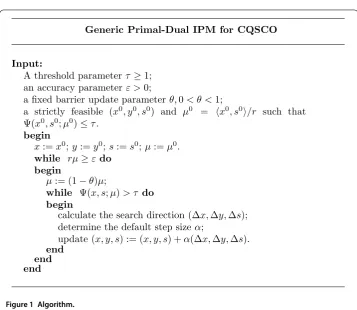
The algorithm considered in this paper is described in Figure .
Given any eligible kernel functionψ(t), the parametersτ,θ and the step sizeαshould be chosen in such a way that the algorithm is ‘optimized’ in the sense that the number of iterations required by the algorithm is as small as possible. We will prove that the resulting iteration bounds depend on the eligible kernel functions in Section .
The purpose of the paper is to propose a unified analysis of kernel-function-based primal-dual IPMs for CQSCO and give a general scheme on how to calculate the it-eration bounds for the entire class of eligible kernel functions. The obtained com-plexity results match the best-known iteration bounds known for large-update meth-ods,O(√rlogrlogεr) and small-update methods,O(√rlogεr). The order of the iteration bounds are derived as good as the ones for the LO case except thatnis replaced byr, the rank of EJA. Although expected, these results were not obvious and, at certain steps of the analysis, they were not trivial and/or straightforward generalization of the LO case. Fur-thermore, this unifies the analysis for a wide class of conic optimization problems, which includes LO, CQO, SOCO, SDO, CQSDO, SCO and so on.
Figure 1 Algorithm.
Section , we uniformly analyze the primal-dual IPMs for CQSCO. In Section , we derive the complexity bounds for large- and small-update methods. In Section , we report some preliminary numerical experiments. Finally, some conclusions and remarks are made in Section .
The following notations are used throughout the paper.Rn,Rn+, andRn++denote the set of all vectors (with ncomponents), the set of non-negative vectors and the set of posi-tive vectors, respecposi-tively.Rm×nis the space of allm×nmatrices.Sn,Sn
+andSn++denote
the cones of symmetric, symmetric positive semidefinite and symmetric positive definite
n×nmatrices, respectively. We use the matrix inner productA•B=tr(ATB),i.e., the trace of the matrixATB. The largest eigenvalue and the smallest eigenvalue ofxare de-fined byλmax(x) andλmin(x), respectively. The Löwner partial ordering ‘K’ ofVdefined
by a symmetric coneK is defined byxKsifx–s∈K. The interior ofKis denoted asintKand we writexKsifx–s∈intK. Finally, ifg(x)≥ is a real-valued function of a real non-negative variable, the notationg(x) =O(x) means thatg(x)≤ ¯cxfor some positive constant¯c, andg(x) =(x) thatcx≤g(x)≤cxfor the two positive constantsc
andc.
2 Preliminaries
For anyx,y∈V, the Lyapunov transformationL(x) and the quadratic representationP(x) are given by
and
P(x) := L(x)–Lx, ()
whereL(x)=L(x)L(x), respectively.
For any EJAV, the corresponding cone of squares
K(V) :=x:x∈V ()
is indeed a symmetric cone (cf.Theorem III.. in []). In the sequel,Kwill always denote a symmetric cone, andVan EJA withrank(V) =rfor whichKis its cone of squares.
The following theorem gives an important decomposition, the spectral decomposition, on the spaceV.
Theorem . (Theorem III.. in []) Let x ∈V. Then there exists a Jordan frame {c, . . . ,cr}and real numbersλ(x), . . . ,λr(x)such that
x= r
i=
λi(x)ci. ()
The numbersλi(x) (with their multiplicities)are called the eigenvalues of x.Furthermore,
the trace and the determinant of x are given by
tr(x) = r
i=
λi(x) and det(x) = r
i=
λi(x),
respectively.
Letx∈Kwith the spectral decomposition given by (), the vector-valued functionψ(x) is defined by
ψ(x) :=ψλ(x)
c+· · ·+ψ
λr(x)cr. ()
Furthermore, if ψ(t) is differentiable, the derivativeψ(t) exists, and we also have the vector-valued functionψ(x), namely
ψ(x) =ψλ(x)
c+· · ·+ψ
λr(x)cr. ()
It should be noted thatψ(x) is just a vector-valued function induced by the derivative ψ(t) of the functionψ(t) rather than the derivative of the vector-valued functionψ(x) defined by ().
The following theorem provides another important decomposition, the Peirce decom-position, on the spaceV.
Theorem .(Theorem IV.. in []) Let x∈Vwith the spectral decomposition given by
().Then we have
V=
where
Vii:={x|x◦ci=x} and Vij:=
xx◦ci=
x=x◦cj
, ≤i<j≤r,
are Peirce spaces ofV.Then,for any x∈V,there exist xi∈R,ci∈Vii,and xij∈Vij(i<j)
such that
x= r
i=
xici+
i<j
xij.
For anyx,s∈V, we define
x,s:=tr(x◦s), ()
and we refer to it as the trace inner product. The Frobenius norm induced by this trace inner product, namely · F, is defined by
xF:=
x,x. ()
Thus, we have
xF=
trx=
r
i=
λ
i(x). ()
Furthermore, we can easily verify that
λmin(x)≤ xF and λmax(x)≤ xF. ()
Lemma .(Lemma in []) Let x,s∈V.Then
λmin(x+s)≥λmin(x) +λmin(s)≥λmin(x) –sF
and
λmax(x+s)≤λmax(x) +λmax(s)≤λmax(x) +sF.
Letf :D→Rbe a univariate function on the open setD⊆Rthat is differentiable or even continuously differentiable if necessary, andx=ri=λi(x)cibe the spectral decom-position ofx∈V with respect to the Jordan frame{c, . . . ,cr}. The real-valued separable spectral functionF:V→Rand the vector-valued separable spectral functionG:V→V are defined by
F(x) := r
i=
and
G(x) := r
i=
fλi(x)ci, ()
respectively.
The following two theorems give explicitly the first derivatives ofF(x) andG(x), respec-tively.
Theorem .(Theorem in []) Let f is continuously differentiable in D.Then F(x)is continuously differentiable at x and
DxF(x) = r
i=
fλi(x)ci.
Theorem .(Lemma in []) Let f is a continuously differentiable in D.Then G(x)is
continuously differentiable at x and
DxG(x) = r
i=
fλi(x)xici+
i<j λi(x)=λj(x)
fλi(x)xij+
i<j λi(x)=λj(x)
f(λi(x)) –f(λj(x)) λi(x) –λj(x)
xij,
where≤i<j≤r.
3 Properties of the eligible kernel (barrier) functions
We call a univariateψ: (,∞)→[,∞) a kernel function [] if it satisfies the following three conditions:
ψ() =ψ() = , (a)
ψ(t) > , (b)
lim
t↓ψ(t) =tlim→∞ψ(t) =∞. (c) This means thatψ(t) is strictly convex and minimal att= , withψ() = . Moreover, (c) implies thatψ(t) has the barrier property.
In this paper, we consider the so-called eligible kernel function [],i.e., the kernel func-tion satisfies four of the following five condifunc-tions, namely the first and the last three con-ditions:
tψ(t) +ψ(t) > , t< , (a)
tψ(t) –ψ(t) > , t> , (b)
ψ(t) < , t> , (c)
Note that the first four conditions are logically independent, and the fifth condition is a consequence of (b) and (c). Since (b) is much simpler to check than (e), in many cases it is easy to know thatψ(t) is eligible if it satisfies the first four conditions [].
The following lemma is cited from [] to state the exponential convexity, which plays an important role in the analysis of kernel-function-based primal-dual IPMs [, ].
Lemma .(Lemma . in []) Let t> and t> .Then
ψ(√tt)≤
ψ(t) +ψ(t)
.
Now, we define the barrier function(v) :intK→R+as
(x,s,μ) :=(v) :=trψ(v). ()
It follows from Theorem . and () that
(v) = r
i=
ψλi(v)
. ()
Furthermore, we have, by Theorem .,
∇(v) =ψ(v) :=ψλ(v)
c+· · ·+ψ
λr(v)
cr, ()
where∇(v) denotes the derivative of the barrier function(v).
As a consequence of Lemma ., we have the following important result.
Theorem .(Theorem .. in []) Let x,s∈intK.Then
P(x)/s/≤
(x) +(s).
Note that during the course of the algorithm the largest values of(v) occur just after the update ofμ. So next we derive an estimate for the effect of aμ-update on the value of (v). It follows from () that
(βv) = r
i=
ψβλi(v).
By applying Theorem . in [], withxbeing the vector inRrconsisting of all the eigen-values of the symmetric conev, the theorem below immediately follows.
Theorem . Let v∈intKandβ≥.Then
(βv)≤rψ
β
(v)
r
.
Corollary . Let≤θ< and v+=√–vθ.If(v)≤τ,then
(v+)≤rψ
(τ r)
√
–θ
Proof Withβ =√
–θ ≥ and(v)≤τ, the corollary follows immediately from
Theo-rem ..
The norm-based proximity measureδ(v) :intK→R+is defined by
δ(v) :=
∇(v)F. ()
It follows from () and () that
δ(v) = ψ
(v)
F=
r
i=
ψλi(v)
. ()
Hence, we can conclude thatδ(v)≥, andδ(v) = if and only if(v) = .
It follows from () and () thatδ(v) and(v) depend only on the eigenvaluesλi(v) of the symmetric coneV. This observation makes it possible to apply Theorem . in [], withxbeing the vector inRrconsisting of all the eigenvalues of the symmetric conev. This gives the following theorem, which yields a lower bound onδ(v) in terms of(v).
Theorem . Let v∈intK.Then
δ(v)≥ ψ
(v).
In what follows, we consider the derivatives of the function(x(t)) with respect tot, wherex(t) =x+tu∈intKwitht∈Randu∈V. It follows from Theorem . and
Theo-rem . that the spectral decomposition ofx(t) with respect to the Jordan frame{c, . . . ,cr} can be defined by
x(t) = r
i=
λi
x(t)ci, ()
and the Peirce decomposition ofucan be defined by
u= r
i=
uici+
i<j
uij. ()
From Theorem . and Theorem ., after some elementary reductions, we can derive the first two derivatives of the general function(x(t)) with respect totas follows:
Dt
x(t)=trDx
x(t)◦x(t)=tr r
i=
ψλi
x(t)ci◦u
()
and
Dtx(t)= r
i=
ψλi
x(t)(ui)+ i<j λi(x(t))=λj(x(t))
ψλi
x(t)tr(uij)
+
i<j λi(x(t))=λj(x(t))
ψ(λi(x(t))) –ψ(λj(x(t))) λi(x(t)) –λj(x(t))
The condition (c) implies thatψ(t) is monotonically decreasing int∈(, +∞). Under the assumption thati<jimpliesλi(x(t))≥λj(x(t)), we can conclude that
Dtx(t)≤ r
i=
ψλi
x(t)(ui)+ i<j
ψλj
x(t)tr(uij), ()
which bounds the second-order derivative of(x(t)) with respect tot(see,e.g., []).
4 Analysis of the algorithms
From () and (), after some elementary reductions, we have
x+=√μP
w(j)/(v+αdx) and s+=√μP(w)–/(v+αds).
Note that during an inner iteration the parameterμis fixed. Hence, after the default step the new scaled vectorv+is given by
v+=P(w+)–/P(w)/(v+αdx) =P(w+)/P(w)–/(v+αds), where, according to Lemma .,
w+=P(x+)/
P(x+)/s+
–/
.
To calculate a decrease of the barrier function(v) during an inner iteration it is stan-dard to consider a decrease as a function ofαdefined by
f(α) :=(v+) –(v).
However, working withf(α) may not be easy because in generalf(α) is not convex. Thus, we are searching for the convex functionf(α) that is an upper bound off(α) and whose
derivatives are easier to calculate than those off(α). The key element in this process is replacingv+with a similar element that will allow the use of exponential-convexity of the
barrier function. By Proposition .. in [], we have
v+∼
P(v+αdx)(v+αds)
and therefore
(v+) =
P(v+αdx)(v+αds) .
Theorem . implies that
(v+)≤
(v+αdx) +(v+αds).
Hence, we have
f(α)≤f(α) :=
which means thatf(α) gives an upper bound for the decrease of the barrier function(v).
Furthermore, we can easily verify thatf() =f() = .
It follows from () that
f(α) =
trψ(v+αdx)◦dx
+trψ(v+αds)◦ds
.
This gives, by (),
f() = tr
ψ(v)◦(dx+ds)
= – tr
ψ(v)◦ψ(v)= – ψ
(v)
F = –δ(v)
< .
Letη=v+αdxandγ =v+αds. To simplify the notations we used (and will use below), the following conventions:
dxi:= (dx)i, dsi:= (ds)i, dxij:= (dx)ij and dsij:= (ds)ij. ()
It follows directly from () and () that
f(α)≤
r
i=
ψλi(η)(dxi)+ i<j
ψλj(η)tr(dxij)
+
r
i=
ψλi(γ)(dsi)+ i<j
ψλj(γ)tr(dsij). ()
In the sequel, we use the short notationδ:=δ(v).
Lemma . One has
dxF+dsF≤δ.
Proof SinceQis a given self-adjoint positive semidefinite linear operator, we have
dx,ds=
dx,Q(dx) –AT(y)=dx,P(w)QP(w)(dx)–dx,AT(y)
=P(w)d
x,Q
P(w)d
x
≥. ()
Hence, we have
δ=dx+dsF=dxF+dsF+ dx,ds ≥ dxF+dsF. ()
This completes the proof of the lemma.
Similar to the proof of Lemma . in [], we have the following lemma, which gives an upper bound off(α) in terms ofδandψ(t).
Lemma . One has
f(α)≤δψλmin(v) – αδ
Letρ(s) : [,∞)→(, ] be the inverse function of –ψ(t) fort≤, whereψ(t) is the eligible kernel function. Similar to the LO case, the default step size is chosen. In this paper, we use
˜
α:=
ψ(ρ(δ)) ()
as the default step size.
In what follows, we will show that the barrier function(v) in each inner iteration with the default step sizeα˜, as defined by (), is decreasing. For this, we need the following technical result.
Lemma .(Lemma . in []) Let h(t)be a twice differentiable convex function with h() = ,h() < and let h(t)attain its(global)minimum at t∗> .If h(t)is increasing for t∈[,t∗],then
h(t)≤th
()
, ≤t≤t
∗.
As a consequence of Lemma . and the fact thatf(α)≤f(α), which is a twice
dif-ferentiable convex function withf() = , andf() = –δ< , we can easily prove the
following lemma.
Lemma . Let the step sizeαsatisfies the conditionα≤ ˜α.Then
f(α)≤–αδ.
Combining the results of Lemma . and (), we have the following theorem, which shows that the default step size () yields a sufficient decrease of the barrier function value during each inner iteration.
Theorem . Letα˜ be the default step size,as given by().Then
f(α˜)≤– δ
ψ(ρ(δ)). ()
By using the condition (d), we can conclude that the right-hand side expression in () is monotonically decreasing inδ(cf.Lemma . in []). Thus, combining the results of Theorems . and ., we have
f(α˜)≤– (ψ
(((v))))
ψ(ρ(ψ(ρ((v))))). ()
This expresses the decrease in(v) during an inner iteration completely inψ, its first and second derivatives, and the inverse functionsρand.
5 Complexity of the algorithms
5.1 Iteration bounds for the algorithms
We need to count how many inner iterations are required to return to the situation where (v)≤τ. We use the value of(v) after theμ-update by, and the subsequent values
in the same outer iteration are denoted ask,k= , , . . . ,K, whereK denotes the total number of inner iterations in the outer iteration.
Let the constantsβ> andγ ∈(, ] be such that for(v)≥τ. We have
(ψ(((v))))
ψ(ρ(ψ(((v)))))≥β(v)
–γ.
Note that the left-hand side expression is increasing in(v). Therefore, such numbersβ andγcertainly exist (take,e.g.,γ = andβequals the value of the left-hand side expression for(v) =τ). In addition, the appropriate values ofβ andγ will vary for each eligible kernel function and finding them may not always be straightforward.
The following lemma provides an estimate for the number of inner iterations between two successive barrier parameter updates, in terms ofand the parametersβandγ.
Lemma . One has
K≤
γ
βγ.
Proof The definition ofKimpliesK–>τ andK≤τand
k+≤k–β(k)–γ, k= , , . . . ,K– .
Thus, the conclusion of the lemma follows immediately from Lemma in [] withtk=k.
This completes the proof of the lemma.
The number of outer iterations coincides with the number of barrier parameterθ up-dates until we obtainrμ<ε. It is well known (cf.Lemma. in []) that the number of outer iterations is bounded above by θlogrε. Thus, an upper bound on the total number of iterations is obtained by multiplying the number of outer iterations and the number of inner iterations.
Theorem . The total number of iterations is bounded above by
γ θβγ log
r
ε.
From Theorem . and Corollary ., we obtain the iteration bound for the algorithm depicted in Figure follows:
θβγ
rψ
(τ r)
√
–θ γ
logr
ε, ()
5.2 Application to the eligible kernel functions
It follows from Theorem . that the iteration bound of the algorithms depends on the pa-rametersβandγ and the upper bound on. Since these are different for different eligible
kernel functions, the iteration bounds will also vary. Similar to the analysis considered in [], Section ., for the LO case, the iteration bounds for large- and small-update methods based on the eligible kernel functions can be performed in a systematic way by using the following scheme.
• Step : Input an eligible kernel functionψ(t); an update parameterθ, <θ< ; a threshold parameterτ; and an accuracy parameterε.
• Step : Solve the equation–
ψ(t) =sto getρ(s), the inverse function of– ψ(t),
t∈(, ]. If the equation is hard to solve, derive a lower bound forρ(s).
• Step : Calculate the decrease of(v)in terms ofδfor the default step sizeα˜ from
f(α˜)≤– δ
ψ(ρ(δ)).
• Step : Solve the equationψ(t) =sto get(s), the inverse function ofψ(t),t≥. If the equation is hard to solve, derive the lower and upper bounds for(s).
• Step : Derive a lower bound forδ(v)in terms of(v)by using
δ(v)≥ ψ
(v).
• Step : Using the results of Step and Step find positive constantsβandγ, with
γ ∈(, ], such that
f(α˜)≤–β(v)–γ.
• Step : Calculate the uniform upper boundfor(v)from
≤Lψ(r,θ,τ) :=rψ
(τ r)
√
–θ
.
• Step : Derive an upper bound for the total number of iterations from
γ θβγ log
r
ε.
• Step : Setτ=O(r)andθ=()so as to calculate an iteration bound for large-update methods, or setτ=O()andθ=(√
r)to get an iteration bound for small-update
methods.
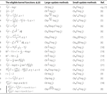
The resulting iteration bounds for a wide class of eligible kernel functions have been out-lined in a series of papers [–, , , –, ] starting with [] for LO, we immediately get the iteration bounds for large- and small-update methods for CQSCO. The resulting iteration bounds are summarized in the rd and th columns of Table . For the detailed analysis of the algorithms can be refereed to the given references.
Remark . For large-update methods, the currently best-known iteration bound is
O
√
rlogrlogr ε
Table 1 Complexity results for the eligible kernel functions
i The eligible kernel functionsψi(t) Large-update methods Small-update methods Ref. 1 t2–1
2 – logt O(rlog
r
ε) O(
√ rlogr
ε) e.g., [1] 2 12(t–1t)2 O(r23logr
ε) O(
√
rlogεr) [6]
3 t2–1 2 +
t1–q–1
q–1 ,q> 1 O(qr q+1
2q logr
ε) O(q2
√ rlogr
ε) [6]
4 t2–1 2 +
t1–q–1 q(q–1) –
q–1
q(t– 1),q> 1 O(qr q+1
2q logr
ε) O(q2
√ rlogr
ε) [5]
5 t2–1 2 +
e 1 t–e
e O(
√
r(logr)2logr
ε) O(
√ rlogr
ε) [6]
6 t2–12 –1te
1
ξ–1dξ O(√r(logr)2logr
ε) O(
√
rlogεr) [6]
7 t2–12 +e q( 1t–1)
–q
q ,q≥1 O(q
√
rlogεr) O(q√qrlogεr) [7]
8 t2–12 –1teq( 1ξ–1)dξ,q≥1 O(q√rlogr
ε) O(q
√qrlogr
ε) [6]
9 t2–12 +(e–1)2e 1 et–1–
e–1
e O(r
3
4logεr) O(√rlogεr) [10]
10 8t2– 11t+ 1 +√2
t– 4 logt O(r 5
6logεr) O(√rlogεr) [19]
11 8t2– 10t+ 2
t3 O(r
5
8logεr) O(√rlogεr) [14]
12 t2–1 2 +
6
πtan (π2+4(1–tt)) O(r 3 4logr
ε) O(
√rlogr
ε) [17]
13 t2–1 2 – log (t) +
1 8tan
2(π(1–t)
2+4t) O(r 2 3logr
ε) O(
√rlogr
ε) [21]
14 p(t2–1)2 +tq–(pqq+1)–1–pqq(+1t–1),p≥1,q> 0 O(√rlogrlogεr) O(√rlogεr) [15]
15 t+1t– 2 O(rlogεr) O(√rlogεr) [9]
16 t– 1 +t1–q–1q–1,q> 1 O(qrlogεr) O(q2√rlogεr) [6]
17 tp+1–1
p+1 – logt,p∈[0, 1] O(rlog r
ε) O(
√rlogr
ε) [18]
18
tp+1–1 p+1 +t
1–q–1
q–1 ,t> 0,p∈[0, 1],q> 1 tp+1–1
p+1 – logt,t> 0,p∈[0, 1],q= 1
O(qr
p+q q(1+p)logr
ε) O(q2
√
rlogεr) [8]
In particular, forψ(t) andψ(t) this bound is obtained if we chooseq=logr, and for
ψ(t) andψ(t) this bound is obtained if we chooseq=logr. The same bound is achieved
forψ(t), also by takingp= andq=logr.
Remark . For small-update methods, the currently best-known iteration bound is
O
√
rlogr ε
.
In particular, forψ(t),ψ(t),ψ(t),ψ(t),ψ(t) andψ(t), this bound is derived is we
takeq=O().
Both for large- and small-update methods, the order of the iteration bounds are obtained as good as the bounds for the LO case except thatnis replaced byr, the rank of the EJA. Thus, the iteration bounds are as good as they can be in the current state-of-the-art.
6 Numerical results
We consider the primal problem of CQSDO in the standard form
min
X•Q(X) +C•X:Ai•X=bi,i= , , . . . ,m,X
,
and its dual problem
max
–
X•Q(X) +b Ty:
m
i=
yiAi–Q(X) +S=C,S
.
Here,Q:Sn→Snis a given self-adjoint positive semidefinite linear operator onSn,i.e., for anyA,B∈Sn,Q(A)•B=A•Q(B) andQ(A)•A≥.b∈Rmis a given vector,C∈Rn×n
is a given matrix. Without loss of generality we assume that the matricesAi,i= , , . . . ,m
are linearly independent and CQSDO satisfy the IPC. The detailed discussion and analysis of primal-dual IPMs for CQSDO can be found in [, , ].
Let us define
P:=XXSX–
X =S–SXSS–, ()
and also we defineD:=P. This leads to the definition of the following variance matrix:
V:=√ μD
–XD–
=√
μDSD . ()
Furthermore, we define the scaled search directions as follows:
DX:=
√μD–XD– and DS:=
√μDSD. ()
The scaled search direction (DX,y,DS) is computed through solving the following linear system:
Ai•DX= , i= , , . . . ,m, m
i=
yiAi–Q(DX) +DS= , ()
DX+DS=V––V,
where
Ai:=
√μDAiD, i= , , . . . ,m and Q(DX) :=DQ(DDXD)D.
Then the new search direction (X,y,S) is obtained from (). If (X,y,S)= (X(μ),y(μ),
S(μ)), then (X,y,S) is nonzero. The new iterate is obtained by taking a default step sizeαalong the search directions as follows:
It should be noted that the default step size () selected during each inner iteration is small enough for analyzing the algorithm, while in practice it should be chosen large enough for the efficiency of the algorithm. In the following test problem, we choose the maximum allowed step size such that the next iterate satisfying the positive semidefinite-ness condition,i.e.,X+αDX andS+αDS.
We consider the following special CQSDO example withQ(X) =E:
A=
⎛ ⎜ ⎜ ⎜ ⎜ ⎜ ⎜ ⎜ ⎜ ⎜ ⎜ ⎜ ⎜ ⎜ ⎝ ⎞ ⎟ ⎟ ⎟ ⎟ ⎟ ⎟ ⎟ ⎟ ⎟ ⎟ ⎟ ⎟ ⎟ ⎠
, A=
⎛ ⎜ ⎜ ⎜ ⎜ ⎜ ⎜ ⎜ ⎜ ⎜ ⎜ ⎜ ⎜ ⎜ ⎝ ⎞ ⎟ ⎟ ⎟ ⎟ ⎟ ⎟ ⎟ ⎟ ⎟ ⎟ ⎟ ⎟ ⎟ ⎠ ,
A=
⎛ ⎜ ⎜ ⎜ ⎜ ⎜ ⎜ ⎜ ⎜ ⎜ ⎜ ⎜ ⎜ ⎜ ⎝ ⎞ ⎟ ⎟ ⎟ ⎟ ⎟ ⎟ ⎟ ⎟ ⎟ ⎟ ⎟ ⎟ ⎟ ⎠
, A=
⎛ ⎜ ⎜ ⎜ ⎜ ⎜ ⎜ ⎜ ⎜ ⎜ ⎜ ⎜ ⎜ ⎜ ⎝ ⎞ ⎟ ⎟ ⎟ ⎟ ⎟ ⎟ ⎟ ⎟ ⎟ ⎟ ⎟ ⎟ ⎟ ⎠ , b= ⎛ ⎜ ⎜ ⎜ ⎝ ⎞ ⎟ ⎟ ⎟
⎠, Q(X) = ⎛ ⎜ ⎜ ⎜ ⎜ ⎜ ⎜ ⎜ ⎜ ⎜ ⎜ ⎜ ⎜ ⎜ ⎝ ⎞ ⎟ ⎟ ⎟ ⎟ ⎟ ⎟ ⎟ ⎟ ⎟ ⎟ ⎟ ⎟ ⎟ ⎠ , C= ⎛ ⎜ ⎜ ⎜ ⎜ ⎜ ⎜ ⎜ ⎜ ⎜ ⎜ ⎜ ⎜ ⎜ ⎝ ⎞ ⎟ ⎟ ⎟ ⎟ ⎟ ⎟ ⎟ ⎟ ⎟ ⎟ ⎟ ⎟ ⎟ ⎠ .
In the test problems, we use the threshold parameterτ = , the accuracy parameter ε= –, and the update parameterθ=
√nwithn= in the implementation. In this case, the algorithm depicted in Figure is indeed a small-update method. We chooseX=E,
point is strictly feasible. The initial value of the barrier parameterμisX•S/nwithn= ,
i.e., . We can easily check that(X,S;μ) = <τ = . So these data can, indeed, be used to initialize our algorithm.
An optimal solution of the primal problem is given by
X∗= ⎛ ⎜ ⎜ ⎜ ⎜ ⎜ ⎜ ⎜ ⎜ ⎜ ⎜ ⎝
. . . . –. –. . –. . . . . . . . . . . . . . –. . –. . . . . . . . –. –. . . . . . . –. –. . –. . . . . .
. . . . . . . . –. . –. –. –. . . .
⎞ ⎟ ⎟ ⎟ ⎟ ⎟ ⎟ ⎟ ⎟ ⎟ ⎟ ⎠
and for the dual problem an optimal solution is given by
y∗= (.; .; .; .),
S∗=
⎛ ⎜ ⎜ ⎜ ⎜ ⎜ ⎜ ⎜ ⎜ ⎜ ⎜ ⎝
. . –. –. . –. –. . . . –. –. . –. . . –. –. . . –. . –. –. –. –. . . –. . –. –. . . –. –. . –. . . –. –. . . –. . –. –. –. . –. –. . –. . .
. . –. –. . –. . . ⎞ ⎟ ⎟ ⎟ ⎟ ⎟ ⎟ ⎟ ⎟ ⎟ ⎟ ⎠
.
The respective objective values are X•Q(X) +C•X= . and –X•Q(X) +
bTy= ., and the duality gapX•Sis .×–, which is less than –.
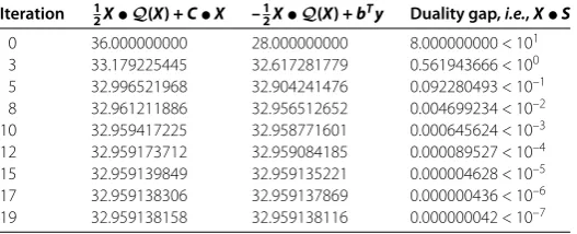
The numerical results of IPM for the sample problem of CQSDO based onψ(t) withθ=
√nare summarized in Table . For our small-update method, we need main iterations to reach our accuracy. To save space, we show the primal and dual objective value at the moments when the duality gap is reduced again with a factor , until the desired accuracy is achieved. The numerical results are summarized in Table .
It is clear from Table that the small-update method presented in this paper is not efficient from a practical point of view, just as the feasible IPMs with the best theoretical performance are far from practical. In fact, our algorithm suffers from the usual drawback of primal-dual IPMs that the number of iterations needed for convergence leads to be close to the upper bound, namely,O(√nlognε). This is due to the small, fixedμ-updates (i.e.,μ+= ( –θ)μwithθ=√n for CQSDO). It is desirable to make the largest possible
[image:19.595.167.431.625.732.2]updateθat each iteration, albeit at the cost of extra computation.
Table 2 Output of IPM for the sample problem of CQSDO based onψ1(t) withθ=2√1n
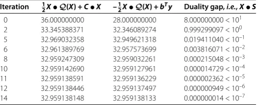
Table 3 Output of IPM for the sample problem of CQSDO based onψ1(t) withθ= 0.9
Iteration 12X•Q(X) +C•X –12X•Q(X) +bTy Duality gap,i.e.,X•S 0 36.000000000 28.000000000 8.000000000 < 101 2 33.345388371 32.346089274 0.999299097 < 100 5 32.969032358 32.949621318 0.019411040 < 10–1 6 32.961389769 32.957573699 0.003816071 < 10–2 8 32.959247309 32.959032261 0.000215048 < 10–3 10 32.959142690 32.959127961 0.000014729 < 10–4 11 32.959138591 32.959136229 0.000002362 < 10–5 12 32.959138446 32.959137497 0.000000949 < 10–6 14 32.959138148 32.959138133 0.000000014 < 10–7
In order to reveal the impact of the update parameterθon the performance of the algo-rithm, we take the larger possible update parameterθ= . in the implementation. In this case, the algorithm depicted in Figure is indeed a large-update method. We only need main iterations to reach our accuracy. The outputs of IPMs for the sample problem of CQSDO based onψ(t) withθ= . are shown in Table .
It is clear from Table that the iteration number of the algorithm depend on the update parameterθ. A larger value of the update parameterθgives rise to better results. However, it should be pointed out that the update parameterθ would be too large to solve the prob-lem in the computational procedure. In the solution procedure, we might use the dynamic updates of the barrier parameter, as described in []. This may significantly enhance the practical performance of the proposed algorithm.
7 Conclusions and remarks
In this paper, we presented a unified approach and comprehensive treatment of primal-dual IPMs for CQSCO based on the entire class of the eligible kernel functions. For large-update methods the best iteration bound isO(√rlogrlogrε) and for small-update meth-ods all iteration bounds have the same order of magnitude, namely,O(√rlogεr), which almost closes the gap between the iteration bounds for large- and small-update methods. Some preliminary numerical results are provided to demonstrate the computational per-formance of the algorithm depicted in Figure .
The paper generalizes results obtained in the following papers, [] where Baiet al. con-sider kernel-based primal-dual IPMs for LO, and [, , ] and [] where Bai et al., El Ghamiet al., Wanget al.and Vieira consider the same type of IPMs for SOCO, SDO, CQSDO and SCO, respectively. It turns out that the iterations bounds are the same as for the non-negative orthant except thatnis replaced byr, the rank of the EJA. However, the analysis of the proposed algorithm is far more complicated in [, , , ]. This is due to the following fact that we lose the orthogonality of search directions that exist in LO, SOCO, SDO, and SCO cases does not hold for CQSCO.
Competing interests
The authors declare that they have no competing interests.
Authors’ contributions
All authors carried out the proof. All authors conceived of the study, and participated in its design and coordination. All authors read and approved the final manuscript.
Author details
1College of Advanced Vocational Technology, Shanghai University of Engineering Science, Shanghai, 201620, P.R. China. 2College of Fundamental Studies, Shanghai University of Engineering Science, Shanghai, 201620, P.R. China.
Acknowledgements
This work was supported by Shanghai Natural Science Fund Project (14ZR1418900), National Natural Science Foundation of China (No. 11001169), China Postdoctoral Science Foundation funded project (Nos. 2012T50427, 20100480604) and Natural Science Foundation of Shanghai University of Engineering Science (No. 2014YYYF01).
Endnote
a It may be worth mentioning that if we use the kernel function of the classical logarithmic barrier function,i.e.,
ψ(t) =1 2(t
2– 1) – logt, thenψ(t) =t–t–1, whence –ψ(v) =v–1–v, and hence system (7) then coincides with the classical system (6).
Received: 29 March 2014 Accepted: 24 July 2014 Published:21 Aug 2014
References
1. Roos, C, Terlaky, T, Vial, JP: Theory and Algorithms for Linear Optimization. An Interior-Point Approach. Wiley, Chichester (1997)
2. Wright, SJ: Primal-Dual Interior-Point Methods. SIAM, Philadelphia (1997) 3. Ye, Y: Interior Point Algorithms: Theory and Analysis. Wiley, Chichester (1997)
4. Anjos, MF, Lasserre, JB: Handbook on Semidefinite, Conic and Polynomial Optimization: Theory, Algorithms, Software and Applications. International Series in Operational Research and Management Science, vol. 166. Springer, New York (2012)
5. Peng, J, Roos, C, Terlaky, T: Self-regular functions and new search directions for linear and semidefinite optimization. Math. Program.93(1), 129-171 (2002)
6. Bai, YQ, El Ghami, M, Roos, C: A comparative study of kernel functions for primal-dual interior-point algorithms in linear optimization. SIAM J. Optim.15(1), 101-128 (2004)
7. Amini, K, Haseli, A: A new proximity function generating the best known iteration bounds for both large-update and small-update interior-point methods. ANZIAM J.49(2), 259-270 (2007)
8. Bai, YQ, Lesaja, G, Roos, C, Wang, GQ, El Ghami, M: A class of large-update and small-update primal-dual interior-point algorithms for linear optimization. J. Optim. Theory Appl.138(3), 341-359 (2008)
9. Bai, YQ, Roos, C: A polynomial-time algorithm for linear optimization based a new simple kernel function. Optim. Methods Softw.18(6), 631-646 (2003)
10. Bai, YQ, Roos, C, El Ghami, M: A primal-dual interior-point method for linear optimization based a new proximity function. Optim. Methods Softw.17(6), 985-1008 (2002)
11. Bai, YQ, Wang, GQ, Roos, C: Primal-dual interior-point algorithms for second-order cone optimization based on kernel functions. Nonlinear Anal.70(10), 3584-3602 (2009)
12. Cai, XZ, Wang, GQ, Zhang, ZH: Complexity analysis and numerical implementation of primal-dual interior-point methods for convex quadratic optimization based on a finite barrier. Numer. Algorithms62(2), 289-306 (2013) 13. Chi, XN, Liu, SY: An infeasible-interior-point predictor-corrector algorithm for the second-order cone program. Acta
Math. Sci.28(3), 551-559 (2008)
14. Cho, GM: Primal-dual interior-point method based on a new barrier function. J. Nonlinear Convex Anal.12(3), 611-624 (2011)
15. Cho, GM: An interior-point algorithm for linear optimization based on a new barrier function. Appl. Math. Comput. 218(2), 386-395 (2011)
16. El Ghami, M, Bai, YQ, Roos, C: Kernel-function based algorithms for semidefinite optimization. RAIRO Oper. Res.43(2), 189-199 (2009)
17. El Ghami, M, Guennounb, ZA, Bouali, S, Steihaug, T: Interior-point methods for linear optimization based on a kernel function with a trigonometric barrier term. J. Comput. Appl. Math.236(15), 3613-3623 (2012)
18. El Ghami, M, Ivanov, ID, Roos, C, Steihag, T: A polynomial-time algorithm for LO based on generalized logarithmic barrier functions. Int. J. Appl. Math.21(1), 99-115 (2008)
19. El Ghami, M, Roos, C: Generic primal-dual interior point methods based on a new kernel function. RAIRO Oper. Res. 42(2), 199-213 (2008)
20. Gu, G, Zangiabadi, M, Roos, C: Full Nesterov-Todd step infeasible interior-point method for symmetric optimization. Eur. J. Oper. Res.214(3), 473-484 (2011)
21. Peyghamia, MR, Hafshejani, SF, Shirvani, L: Complexity of interior-point methods for linear optimization based on a new trigonometric kernel function. J. Comput. Appl. Math.255(1), 74-85 (2014)
22. Tang, JY, He, GP, Fang, L: A new kernel function and its related properties for second-order cone optimization. Pac. J. Optim.8(2), 321-346 (2012)
23. Vieira, MVC: Jordan algebraic approach to symmetric optimization. PhD thesis, Electrical Engineering, Mathematics and Computer Science, Delft University of Technology, The Netherlands (2007)
24. Wang, GQ, Bai, YQ, Roos, C: Primal-dual interior-point algorithms for semidefinite optimization based on a simple kernel function. J. Math. Model. Algorithms4(4), 409-433 (2005)
26. Wang, GQ, Bai, YQ: A class of polynomial interior-point algorithms for the CartesianP-matrix linear complementarity problem over symmetric cones. J. Optim. Theory Appl.152(3), 739-772 (2012)
27. Wang, GQ, Bai, YQ: A new full Nesterov-Todd step primal-dual path-following interior-point algorithm for symmetric optimization. J. Optim. Theory Appl.154(3), 966-985 (2012)
28. Toh, KC: An inexact primal-dual path following algorithm for convex quadratic SDP. Math. Program.112(1), 221-254 (2008)
29. Li, L, Toh, KC: A polynomial-time inexact interior-point method for convex quadratic symmetric cone programming. J. Math-for-Ind.2B, 199-212 (2010)
30. Wang, GQ, Zhu, DT: A unified kernel function approach to primal-dual interior-point algorithms for convex quadratic SDO. Numer. Algorithms57(4), 537-558 (2011)
31. Wang, GQ, Zhang, ZH, Zhu, DT: On extending primal-dual interior-point method for linear optimization to convex quadratic symmetric cone optimization. Numer. Funct. Anal. Optim.34(5), 576-603 (2012)
32. Wang, GQ, Yu, CJ, Teo, KL: A full Nesterov-Todd step feasible interior-point method for convex quadratic optimization over symmetric cone. Appl. Math. Comput.221(15), 329-343 (2013)
33. Bai, YQ, Zhang, LP: A full-Newton step interior-point algorithm for symmetric cone convex quadratic optimization. J. Ind. Manag. Optim.7(4), 891-906 (2011)
34. Achache, M: A full Nesterov-Todd step feasible primal-dual interior point algorithm for convex quadratic semi-definite optimization. Appl. Math. Comput.231(1), 581-590 (2014)
35. Faybusovich, L: Euclidean Jordan algebras and interior-point algorithms. Positivity1(4), 331-357 (1997) 36. Schmieta, SH, Alizadeh, F: Extension of primal-dual interior-point algorithms to symmetric cones. Math. Program.
96(3), 409-438 (2003)
37. Nesterov, YE, Todd, MJ: Self-scaled barriers and interior-point methods for convex programming. Math. Oper. Res. 22(1), 1-42 (1997)
38. Nesterov, YE, Todd, MJ: Primal-dual interior-point methods for self-scaled cones. SIAM J. Optim.8(2), 324-364 (1998) 39. Faybusovich, L: A Jordan-algebraic approach to potential-reduction algorithms. Math. Z.239(1), 117-129 (2002) 40. Faraut, J, Korányi, A: Analysis on Symmetric Cone. Oxford University Press, New York (1994)
41. Baes, M: Convexity and differentiability properties of spectral functions and spectral mappings on Euclidean Jordan algebras. Linear Algebra Appl.422(2-3), 664-700 (2007)
42. Korányi, A: Monotone functions on formally real Jordan algebras. Math. Ann.269(1), 73-76 (1984)
10.1186/1029-242X-2014-308