A scaled three term conjugate gradient method for unconstrained optimization

(1)

R E S E A R C H

Open Access

A scaled three-term conjugate gradient

method for unconstrained optimization

Ibrahim Arzuka

*

_{, Mohd R Abu Bakar and Wah June Leong}

*_{Correspondence:}

[email protected] Institute for Mathematical Research, Universiti Putra Malaysia, Serdang, Selangor 43400, Malaysia

Abstract

Conjugate gradient methods play an important role in many fields of application due to their simplicity, low memory requirements, and global convergence properties. In this paper, we propose an efficient three-term conjugate gradient method by utilizing the DFP update for the inverse Hessian approximation which satisfies both the sufficient descent and the conjugacy conditions. The basic philosophy is that the DFP update is restarted with a multiple of the identity matrix in every iteration. An acceleration scheme is incorporated in the proposed method to enhance the reduction in function value. Numerical results from an implementation of the proposed method on some standard unconstrained optimization problem show that the proposed method is promising and exhibits a superior numerical performance in comparison with other well-known conjugate gradient methods.

Keywords: unconstrained optimization; nonlinear conjugate gradient method; quasi-Newton methods

1 Introduction

In this paper, we are interested in solving nonlinear large scale unconstrained optimization problems of the form

minf(x), x∈ n, ()

wheref :n_→_{is an at least twice continuously diﬀerentiable function. A nonlinear} conjugate gradient method is an iterative scheme that generates a sequence{xk} of an approximation to the solution of (), using the recurrence

xk+=xk+αkdk, k= , , , , . . . , ()

whereαk>  is the steplength determined by a line search strategy which either mini-mizes the function or reduces it suﬃciently along the search direction anddkis the search direction deﬁned by

dk= ⎧ ⎨ ⎩

–gk; k= ,

–gk+βkdk–; k≥,

(2)

wheregkis the gradient off at a pointxkandβkis a scalar known as the conjugate gradient parameter. For example, Fletcher and Reeves (FR) [], Polak-Ribiere-Polyak (PRP) [], Liu and Storey (LS) [], Hestenes and Stiefel (HS) [], Dai and Yuan (DY) [] and Fletcher (CD) [] used an update parameter, respectively, given by

β_kFR= g T kgk gT

k–gk–

, β_kPRP= g T kyk–

gT k–gk–

, β_kLS=–g T kyk–

dT k–gk–

,

β_kHS= g T kyk–

dT k–yk–

, β_kDY= g T kgk dT

k–yk–

, β_kCD= – g T kgk dT

k–yk–

,

whereyk–=gk–gk–. If the objective function is quadratic, with an exact line search the

performances of these methods are equivalent. For a nonlinear objective function different βklead to a different performance in practice. Over the years, after the practical conver-gence result of Al-Baali [] and later of Gilbert and Nocedal [] attention of researchers has been on developing on conjugate gradient methods that possesses the sufficient descent condition

g_kTdk≤–cgk, ()

for some constantc> . For instance the CG-DESCENT of Hager and Zhang []

β_kHZ=maxβ_kN,ηk

, ()

where

β_kN=  dT

k–yk–

yk–– dk–

yk–

dT k–yk–

T gk

and

ηk=

–

dk–min{gk–,η}

,

which is based on the modiﬁcation of HS method. Another important class of conju-gate gradient methods is the so-called three-term conjuconju-gate gradient method in which the search direction is determined as a linear combination ofgk,sk, andykas

dk= –gk–τsk+τyk, ()

whereτandτare scalar. Among the generated three-term conjugate gradient methods in

the literature we have the three-term conjugate methods proposed by Zhanget al.[, ] by considering a descent modiﬁed PRP and also a descent modiﬁed HS conjugate gradient method as

dk+= –gk++

gT k+yk

g_kTgk

dk–

gT k+dk

g_kTgk

(3)

and

dk+= –gk++

g_kT_+yk sT

kyk

sk–

g_kT_+sk sT

kyk

yk,

wheresk=xk+–xk. An attractive property of these methods is that at each iteration, the

search direction satisﬁes the descent condition, namelygT

kdk= –cgkfor some constant c> . In the same manner, Andrei [] considers the development of a three-term conju-gate gradient method from the BFGS updating scheme of the inverse Hessian approxima-tion restarted as an identity matrix at every iteraapproxima-tion where the search direcapproxima-tion is given by

dk+= –gk++

yT kgk+

yT ksk

–

y– yk



yT ksk

T_sT kgk+

yT ksk

sk–

sT kgk+

yT ksk

yk.

An interesting feature of this method is that both the sufficient and the conjugacy condi-tions are satisfied and we have global convergence for a uniformly convex function. Mo-tivated by the good performance of the three-term conjugate gradient method, we are interested in developing a three-term conjugate gradient method which satisfies both the sufficient descent condition, the conjugacy condition, and global convergence. The re-maining part of this paper is structured as follows: Section  deals with the derivation of the proposed method. In Section , we present the global convergence properties. The numerical results and discussion are reported in Section . Finally, a concluding remark is given in the last section.

2 Conjugate gradient method via memoryless quasi-Newton method

In this section, we describe the proposed method which would satisﬁed both the suﬃcient descent and the conjugacy conditions. Let us consider the DFP method, which is a Newton method belonging to the Broyden class []. The search direction in the quasi-Newton methods is given by

dk= –Hkgk, ()

whereHkis the inverse Hessian approximation updated by the Broyden class. This class consists of several updating schemes, the most famous being the BFGS and the DFP; ifHk is updated by the DFP then

Hk+=Hk+ sksTk sT

kyk

–Hkyky T kHk yT

kHkyk

, ()

such that the secant equation

Hk+yk=sk ()

(4)

solving (), where at every step the inverse Hessian approximation is updated as an iden-tity matrix. Thus, the search direction can be determined without requiring the storage of any matrix. It was proposed by Shanno [] and Perry []. The classical conjugate gradi-ent methods PRP [] and FR [] can be seen as memoryless BFGS (see Shanno []). We proposed our three-term conjugate gradient method by incorporating the DFP updating scheme of the inverse Hessian approximation (), within the frame of a memoryless quasi-Newton method where at each iteration the inverse Hessian approximation is restarted as a multiple of the identity matrix with a positive scaling parameter as

Qk+=μkI+ sksT_k sT_kyk

–μk ykyT_k yT_kyk

, ()

and thus, the search direction is given by

dk+= –Qk+gk+= –μkgk+–

sT kgk+

sT_kyk sk+μk

yT kgk+

yT_kyk

yk. ()

Various strategies can be considered in deriving the scaling parameterμk; we prefer the following which is due to Wolkowicz []:

μk= sT_ksk yT

ksk – s

T ksk yT

ksk 

– s T ksk yT

kyk

. ()

The new search direction is then given by

dk+= –μkgk+–ϕsk+ϕyk, ()

where

ϕ=

sT_kgk+

sT kyk

()

and

ϕ=μk yT

kgk+

yT kyk

. ()

We present the algorithm of the proposed method as follows.

2.1 Algorithm (STCG)

In this section, we present the algorithm of the proposed method. It has been reported that the line search in conjugate gradient method performs more function evaluations so as to obtain a desirable steplengthαkdue to poor scaling of the search direction (see Nocedal []). As a consequence, we incorporate the acceleration scheme proposed by Andrei [], so as to have some reduction in the function evaluations. The new approximation to the minimum instead of () is determined by

xk+=xk+αkϑkdk, ()

(5)

Algorithm 

Step . Select an initial pointxoand determinef(xo)andg(xo). Setdo= –goandk= . Step . Test the stopping criteriongk ≤, if satisﬁed stop. Else go to Step . Step . Determine the steplengthαkas follows:

Givenδ∈(, )andp,p, with <p<p< .

(i) Setα= . (ii) Test the relation

f(x+αdk) –f(xk)≤αδg_kTdk. ()

(iii) If () is satisﬁed, thenαk=αand go to Step  else choose a new α∈[pα,pα]and go to (ii).

Step . Determinez=xk+αkdk, computegz=∇f(z)andyk=gk–gz. Step . Determinerk=αkgkTdkandqk= –αkyTkdk.

Step . Ifqk= , thenϑk=_qrk

k,xk+=xk+ϑkαkdkelsexk+=xk+αkdk.

Step . Determine the search directiondk+by () whereμk,ϕ, andϕare computed by

(), (), and (), respectively. Step . Setk:=k+ and go to Step .

3 Convergence analysis

In this section, we analyze the global convergence of the propose method, where we as-sume thatgk =  for allk≥ else a stationary point is obtained. First of all, we show that the search direction satisﬁes the suﬃcient descent and the conjugacy conditions. In order to present the results, the following assumptions are needed.

Assumption  The objective functionf is convex and the gradientgis Lipschitz contin-uous on the level set

K=x∈ n|f(x)≤f(x)

. ()

Then there exist some positive constantsψ,ψ, andLsuch that

g(x) –g(y)≤Lx–y ()

and

ψz≤zTG(x)z≤ψz, ()

for allz∈Rnandx,y∈KwhereG(x) is the Hessian matrix off. Under Assumption , we can easily deduce that

ψsk≤sTkyk≤ψsk, ()

wheresT

kyk=sTkGs¯ kandG¯ = 

G(xk+λsk)skdλ. We begin by showing that the updating

(6)

Lemma . Suppose that Assumptionholds;then the matrix()is positive deﬁnite.

Proof In order to show that the matrix () is positive deﬁnite we need to show thatμkis well deﬁned and bounded. First, by the Cauchy-Schwarz inequality we have

sT_ksk yT

ksk 

– s T ksk yT

kyk =(s

T

ksk)((sTksk)(ykTyk) – (yTksk)) (yT

ksk)(yTkyk) ≥,

and this implies that the scaling parameterμkis well deﬁned. It follows that

 <μk=s T ksk yT

ksk –

sT_ksk yT

ksk 

– s T ksk yT

kyk 



≤ sTksk yT

ksk

≤ sk ψ_sk =

 ψ_.

When the scaling parameter is positive and bounded above, then for any non-zero vector p∈ n_{we obtain}

pTQk+p=μkpTpI+ pT_s

ksTkp sT

kyk –μk

pT_y kyTkp yT

kyk

=μk

(pT_p₎₍_yT

kyk) –pTykyTkp yT_kyk

+(p

T_s_k)

sT_kyk .

By the Cauchy-Schwarz inequality and (), we have (pT_p₎₍_yT

kyk) – (pTyk)(yTkp)≥ and yT

ksk> , which implies that the matrix () is positive deﬁnite∀k≥. Observe also that

tr(Qk+) =tr(μkI) + sT_ksk sT

kyk –μk

yT_kyk yT

kyk

= (n– )μk+ sT_ksk sT

kyk

≤n–  ψ_ +

sk

ψsk

=ψ+n– 

ψ_ . ()

Now,

 <  ψ≤

sT_ksk yT

ksk

≤tr(Qk+)≤

ψ+n– 

ψ_ . ()

Thus,tr(Qk+) is bounded. On the other hand, by the Sherman-Morrison House-Holder

formula (Q–_k_+ is actually the memoryless updating matrix updated from _μ

kI using the direct DFP formula), we can obtain

Q–_k_+=  μk

I–  μk

yksT_k +skyT_k sT_kyk

+

 +  μk

sT ksk sT_kyk

ykyT_k sT_kyk

(7)

We can also establish the boundedness oftr(Q–

k+) as

trQ–_k_+=tr  μk I –  μk sT

kyk sT_kyk

+yk



sT_kyk + 

μk

skyk (sT_kyk)

≤ n μk

–  μk

+L

_s_k

ψsk

+  μk

L_s_k

ψ_sk

≤(n– ) ψ  +L  ψ + L  ψ 

=ω, ()

whereω=(n_ψ–) 

+L

ψ +

L

ψ_> , forn≥.

Now, we shall state the suﬃcient descent property of the proposed search direction in the following lemma.

Lemma . Suppose that Assumptionholds on the objective function f then the search direction()satisﬁes the suﬃcient descent condition gT

k+dk+≤–cgk+.

Proof Since –gT

k+dk+ ≥ _tr₍_Q–

k+)

gk+ (see for example Leong [] and Babaie-Kafaki

[]), then by using () we have

–g_kT_+dk+≥cgk+, ()

wherec=min{,

ω}. Thus,

g_kT_+dk+≤–cgk+. ()

Dai-Liao [] extended the classical conjugacy condition fromyT

kdk+=  to

yT_kdk+= –t

sT_kgk+

, ()

wheret≥. Thus, we can also show that our proposed method satisﬁes the above

conju-gacy condition.

Lemma . Suppose that Assumptionholds,then the search direction()satisﬁes the conjugacy condition().

Proof By (), we obtain

yT_kdk+= –μyTkgk+–

sT kgk+ sT_kyk

yT_ksk+μ yT

kgk+ yT_kyk

yT_kyk

= –μyT_kgk+–

sT kgk+ sT_kyk

sT_kyk+μ yT

kgk+ yT_kyk

yT_kyk

= –μyT_kgk+–sTkgk++μyTkgk+

(8)

where the result holds fort= . The following lemma gives the boundedness of the search

direction.

Lemma . Suppose that Assumptionholds then there exists a constant p> such that dk+ ≤Pgk+,where dk+is deﬁned by().

Proof A direct result of () and the boundedness oftr(Qk+) gives

dk+=Qk+gk+

≤tr(Qk+)gk+

≤Pgk+, ()

whereP= (ψ_ψ+n– 

).

In order to establish the convergence result, we give the following lemma.

Lemma . Suppose that Assumptionholds.Then there exist some positive constantsγ

andγsuch that for any steplengthαkgenerated by Stepof Algorithmwill satisfy either of the following:

f(xk+αkdk) –f(xk)≤

–γ(gkTdk)

dk , ()

or

f(xk+αkdk) –f(xk)≤γgkTdk. ()

Proof Suppose that () is satisﬁed withαk= , then

f(xk+αkdk) –f(xk)≤δgkTdk, ()

implies that () is satisﬁed withγ=δ.

Supposeαk< , and that () is not satisﬁed. Then for a steplengthα≤α_pk_ we have

f(xk+αdk) –f(xk) >δαgkTdk. ()

Now, by the mean-value theorem there exists a scalarτk∈(, ) such that

f(xk+αdk) –f(xk) =αg(xk+τ αdk)Tdk. ()

From () we have

(δ– )αgT_kdk<α

g(xk+τkαdk) –gk T

dk

=αyT_kdk

(9)

which implies

α≥–( –δ)(g T kdk)

Ldk . ()

Now,

αk≥pα≥–

( –δ)(g_kTdk)

Ldk . ()

Substituting () in () we have the following:

f(xk+αkdk) –f(xk)≤–

δ( –δ)(gT kdk) Ldk

g_kTdk

=–γ(g T kdk) dk ,

where

γ=

δ( –δ)

L .

Therefore

–γ(gkTdk)

dk . ()

Theorem . Suppose that Assumptionholds.Then Algorithmgenerates a sequence of approximation{xk}such that

lim

k→∞gk= . ()

Proof As a direct consequence of Lemma ., the suﬃcient descent property (), and the boundedness of the search direction () we have

–γ(gkTdk) dk

≤–γcgk

P_g_k

=–γc



P gk

 _()

or

f(xk+αkdk) –f(xk)≤γgkTdk

(10)

Hence, in either case, there exists a positive constantγsuch that

f(xk+αkdk) –f(xk)≤–γgk. ()

Since the steplengthαkgenerated by Algorithm  is bounded away from zero, () and () imply thatf(xk) is a non-increasing sequence. Thus, by the boundedness off(xk) we have

 = lim k→∞

f(xk+) –f(xk)

≤–γ lim

k→∞gk

_,

and as a result

lim

k→∞gk= . ()

4 Numerical results

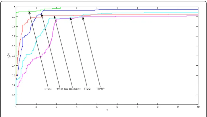
In this section, we present the results obtained from the numerical experiment of our proposed method in comparison with the CG-DESCENT (CG-DESC) [], three-term Hestenes-Stiefel (TTHS) [], three-term Polak-Ribiere-Polyak (TTPRP) [], and TTCG [] methods. We evaluate the performance of these methods based on iterations and function evaluations. By considering some standard unconstrained optimization test problems obtained from Andrei [], we conducted ten numerical experiments for each test function with the size of the variable ranging from ≤n≤,. The algo-rithms were implemented using Matlab subroutine programming on a PC (Intel(R) core(TM) Duo E . GHz  GB) -bit Operating system. The program termi-nates whenever gk< where = –_{or a method failed to converges within ,}

(11)

[image:11.595.117.478.81.284.2]

Figure 1 Performance proﬁles based on iterations.

Figure 2 Performance proﬁles based on function evaluations.

5 Conclusion

[image:11.595.118.477.348.544.2]

(12)

[image:12.595.115.478.144.704.2]

Appendix

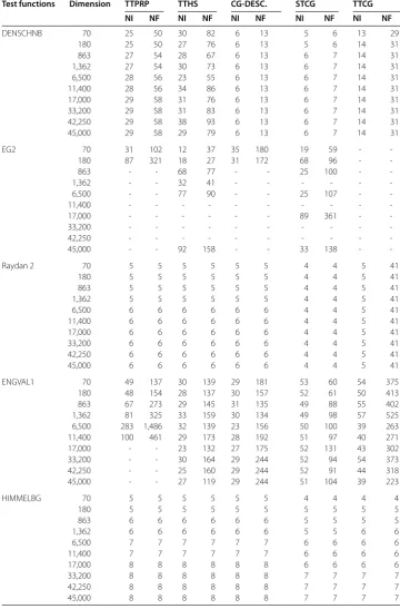
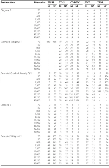
Table 1 Numerical results of TTPRP, TTHS, CG-DESCENT, STCG, and TTCG

Test functions Dimension TTPRP TTHS CG-DESC. STCG TTCG

NI NF NI NF NI NF NI NF NI NF

Extended BD1 70 27 73 39 142 28 102 19 31 25 133

180 28 77 50 207 28 102 19 31 26 157

863 31 85 51 194 31 124 20 33 26 157

1,362 31 85 65 259 31 124 20 33 26 157

6,500 31 85 37 144 31 124 20 33 28 164

11,400 31 85 52 216 31 124 20 33 28 164

17,000 31 85 55 215 31 124 20 33 28 164

33,200 32 88 59 249 31 124 21 34 28 164

42,250 32 88 56 205 31 124 - - 28 164

45,000 32 88 58 220 31 124 22 37 28 164

Extended Rosenbrock 70 44 227 23 156 55 590 125 156 87 828

180 52 272 40 264 42 349 119 186 129 1,243

863 55 285 41 290 33 269 100 136 115 1,098

1,362 60 315 46 323 28 230 91 142 -

-6,500 62 326 22 143 27 220 103 147 -

-11,400 74 401 23 159 27 209 116 191 -

-17,000 82 436 22 143 30 236 111 141 -

-33,200 62 322 39 240 28 213 83 125 -

-42,250 67 355 21 155 29 223 133 157 -

-45,000 75 393 22 158 22 174 134 157 -

-Diagonal 7 70 11 22 4 40 4 52 3 4 6 18

180 11 22 4 40 4 52 3 4 6 18

863 12 24 4 40 4 52 3 4 6 18

1,362 12 24 4 40 4 52 3 4 6 18

6,500 12 24 4 40 4 52 4 5 6 18

11,400 12 24 4 40 4 52 4 5 6 18

17,000 34 53 4 40 4 52 4 5 6 18

33,200 - - 4 40 4 52 4 5 6 18

42,250 - - 4 40 4 52 4 5 6 18

45,000 - - 4 40 4 52 4 5 6 18

DENSCHNF 70 25 126 47 403 20 171 6 17 15 126

180 25 126 49 420 20 171 6 18 16 136

863 27 136 50 429 21 179 7 18 16 135

1,362 27 136 52 446 22 188 7 18 16 135

6,500 28 141 53 455 22 188 19 31 16 135

11,400 28 141 53 455 22 188 19 31 16 135

17,000 29 146 53 455 22 188 19 31 16 135

33,200 29 146 54 463 22 188 19 31 16 135

42,250 29 146 54 463 22 188 19 31 16 135

45,000 29 146 55 472 22 188 19 31 16 135

Extended Himmelblau 70 34 135 20 126 19 114 9 15 18 124

180 36 143 16 85 19 114 9 15 18 124

863 36 143 15 76 18 121 9 15 18 124

1,362 37 147 12 75 18 121 9 15 18 124

6,500 38 151 9 54 19 128 9 15 20 137

11,400 39 155 11 78 19 128 9 15 20 137

17,000 39 155 12 76 19 128 9 15 20 137

33,200 40 159 24 152 19 128 9 15 20 137

42,250 40 159 16 136 19 128 9 15 20 137

(13)

Table 1 (Continued)

DQDRTIC 70 5 5 5 24 5 36 - - 43 362

180 5 5 5 27 5 35 - - 46 391

863 5 5 5 31 5 35 - - 44 371

1,362 5 5 5 29 5 35 - - 46 395

6,500 5 5 5 28 5 35 - - 111 961

11,400 5 5 5 24 5 35 - - 60 516

17,000 5 5 5 33 5 35 - - 37 320

33,200 5 5 5 26 5 35 - - 59 516

42,250 5 5 5 29 5 35 - - 64 548

45,000 5 5 5 27 5 35 - - 55 462

HIMMELH 70 - - - 7 7 23 80

180 - - - 7 7 18 54

863 - - - 7 7 23 70

1,362 - - - 7 7 22 77

6,500 - - - 7 7 23 83

11,400 - - - 7 7 28 71

17,000 - - - 7 7 22 65

33,200 - - - 7 7 33 90

42,250 - - - 7 7 29 89

45,000 - - - 7 7 26 91

Extended BD2 70 30 96 19 73 9 37 13 23 36 237

180 31 100 22 87 9 37 13 23 39 254

863 34 110 11 50 10 43 13 23 41 264

1,362 34 110 11 44 10 43 13 23 43 276

6,500 35 114 12 40 10 40 13 23 42 272

11,400 36 118 25 66 10 43 13 23 43 273

17,000 36 118 18 70 10 43 13 23 36 231

33,200 37 122 10 45 10 48 13 23 39 246

42,250 37 122 17 71 10 38 13 23 37 237

45,000 37 122 9 39 10 38 13 23 37 236

Extended Maratos 70 25 135 23 60 26 86 37 103 109 934

180 25 143 24 63 26 86 37 103 107 895

863 27 143 24 63 26 86 38 104 102 871

1,362 27 147 33 82 - - 38 104 112 887

6,500 27 151 94 209 - - 38 104 121 1,034

11,400 120 308 110 246 - - 38 104 118 949

17,000 278 681 102 229 - - 38 104 119 1,004

33,200 - - 140 302 - - 38 104 96 814

42,250 - - 140 302 - - 38 104 105 867

45,000 - - 159 350 - - 38 104 92 787

NONDIA 70 8 52 - - 12 141 12 37 34 441

180 11 83 - - 14 170 18 27 -

-863 14 119 - - 23 337 68 77 -

-1,362 11 96 - - 26 389 32 41 -

-6,500 16 155 - - 1,029 1,555 77 90 -

-11,400 16 167 - - - - 161 185 -

-17,000 16 168 - - -

-33,200 16 168 - - -

-42,250 21 234 - - -

[image:13.595.117.476.127.675.2]

(14)

-Table 1 (Continued)

DENSCHNB 70 25 50 30 82 6 13 5 6 13 29

180 25 50 27 76 6 13 5 6 14 31

863 27 54 28 67 6 13 6 7 14 31

1,362 27 54 30 73 6 13 6 7 14 31

6,500 28 56 23 55 6 13 6 7 14 31

11,400 28 56 34 86 6 13 6 7 14 31

17,000 29 58 31 76 6 13 6 7 14 31

33,200 29 58 31 83 6 13 6 7 14 31

42,250 29 58 38 93 6 13 6 7 14 31

45,000 29 58 29 79 6 13 6 7 14 31

EG2 70 31 102 12 37 35 180 19 59 -

-180 87 321 18 27 31 172 68 96 -

-863 - - 68 77 - - 25 100 -

-1,362 - - 32 41 - - -

-6,500 - - 77 90 - - 25 107 -

-11,400 - - -

-17,000 - - - 89 361 -

-33,200 - - -

-42,250 - - -

-45,000 - - 92 158 - - 33 138 -

-Raydan 2 70 5 5 5 5 5 5 4 4 5 41

180 5 5 5 5 5 5 4 4 5 41

863 5 5 5 5 5 5 4 4 5 41

1,362 5 5 5 5 5 5 4 4 5 41

6,500 6 6 6 6 6 6 4 4 5 41

11,400 6 6 6 6 6 6 4 4 5 41

17,000 6 6 6 6 6 6 4 4 5 41

33,200 6 6 6 6 6 6 4 4 5 41

42,250 6 6 6 6 6 6 4 4 5 41

45,000 6 6 6 6 6 6 4 4 5 41

ENGVAL1 70 49 137 30 139 29 181 53 60 54 375

180 48 154 28 137 30 157 52 61 50 413

863 67 273 29 145 31 135 49 88 55 402

1,362 81 325 33 159 30 134 49 98 57 525

6,500 283 1,486 32 139 23 156 50 100 39 263

11,400 100 461 29 173 28 192 51 97 40 271

17,000 - - 23 132 27 175 52 131 43 302

33,200 - - 30 164 29 244 52 94 54 373

42,250 - - 25 160 29 244 52 91 44 318

45,000 - - 27 119 29 244 51 104 39 223

HIMMELBG 70 5 5 5 5 5 5 4 4 4 4

180 5 5 5 5 5 5 5 5 5 5

863 6 6 6 6 6 6 5 5 5 5

1,362 6 6 6 6 6 6 5 5 6 6

6,500 7 7 7 7 7 7 6 6 6 6

11,400 7 7 7 7 7 7 6 6 6 6

17,000 8 8 8 8 8 8 6 6 6 6

33,200 8 8 8 8 8 8 7 7 7 7

42,250 8 8 8 8 8 8 7 7 7 7

[image:14.595.116.477.128.676.2]

(15)

Table 1 (Continued)

Diagonal 5 70 4 4 4 4 4 4 4 4 3 21

180 4 4 4 4 4 4 4 4 3 21

863 4 4 4 4 4 4 4 4 3 21

1,362 4 4 4 4 4 4 4 4 3 21

6,500 4 4 4 4 4 4 4 4 3 21

11,400 4 4 4 4 4 4 4 4 4 22

17,000 4 4 4 4 4 4 4 4 4 22

33,200 4 4 4 4 4 4 4 4 4 22

42,250 4 4 4 4 4 4 4 4 4 22

45,000 4 4 4 4 4 4 4 4 4 22

Extended Tridigonal 1 70 343 465 19 24 19 24 22 40 17 51

180 - - 21 24 20 24 22 40 20 51

863 - - 21 25 21 26 28 46 20 61

1,362 - - 22 29 21 26 28 46 20 61

6,500 - - 23 30 23 28 31 55 21 97

11,400 - - 23 30 23 28 31 56 21 97

17,000 - - 20 34 23 28 32 50 21 97

33,200 - - 23 44 24 29 31 49 21 97

42,250 - - 22 27 24 29 42 63 21 97

45,000 - - 22 38 24 29 46 64 21 97

Extended Quadratic Penalty QP1 70 8 25 10 53 7 33 7 15 15 99

180 9 36 10 53 6 21 9 18 18 124

863 12 44 11 58 6 25 12 24 21 154

1,362 8 32 8 48 8 49 13 25 16 135

6,500 13 48 10 51 12 121 14 32 69 796

11,400 11 43 15 107 30 328 15 32 188 976

17,000 7 26 11 52 58 702 15 30 381 1,616

33,200 12 55 13 85 231 2,500 16 43 -

-42,250 13 52 10 61 381 2,950 16 43 -

-45,000 8 39 10 61 433 3,584 15 33 -

-Diagonal 8 70 9 18 4 9 3 7 3 5 4 33

180 9 18 4 9 3 7 3 5 4 33

863 10 20 4 10 4 9 3 5 4 33

1,362 10 20 4 12 4 10 3 5 4 33

6,500 10 20 4 10 4 8 3 5 4 33

11,400 10 20 4 10 4 8 3 5 4 33

17,000 10 20 4 12 4 8 3 5 4 33

33,200 13 24 4 11 4 8 3 5 4 33

42,250 23 36 4 10 4 8 3 5 4 33

45,000 23 36 4 10 4 8 3 5 4 33

Extended Tridigonal 2 70 44 155 13 25 19 24 18 23 17 68

180 45 157 20 22 20 25 18 23 20 84

863 42 146 21 43 21 26 17 21 20 84

1,362 42 146 20 27 21 26 17 21 20 84

6,500 42 146 22 26 23 28 17 22 21 97

11,400 42 146 20 27 23 28 17 22 21 97

17,000 42 146 23 27 23 28 17 22 21 97

33,200 41 143 23 25 24 29 17 22 21 97

42,250 41 143 24 51 24 29 17 22 21 97

45,000 41 143 25 50 24 29 17 22 21 97

Competing interests

We hereby declare that there are no competing interests with regard to the manuscript.

Authors’ contributions

We all participated in the establishment of the basic concepts, the convergence properties of the proposed method and in the experimental result in comparison of the proposed method with order existing methods.

[image:15.595.115.478.95.653.2]

(16)

References

1. Fletcher, R, Reeves, CM: Function minimization by conjugate gradients. Comput. J.7(2), 149-154 (1964)

2. Polak, E, Ribiere, G: Note sur la convergence de méthodes de directions conjuguées. ESAIM: Mathematical Modelling and Numerical Analysis - Modélisation Mathématique et Analyse Numérique3(R1), 35-43 (1969)

3. Liu, Y, Storey, C: Eﬃcient generalized conjugate gradient algorithms, part 1: theory. J. Optim. Theory Appl.69(1), 129-137 (1991)

4. Hestenes, MR: The conjugate gradient method for solving linear systems. In: Proc. Symp. Appl. Math VI, American Mathematical Society, pp. 83-102 (1956)

5. Dai, Y-H, Yuan, Y: A nonlinear conjugate gradient method with a strong global convergence property. SIAM J. Optim. 10(1), 177-182 (1999)

6. Fletcher, R: Practical Methods of Optimization. John Wiley & Sons, New York (2013)

7. Al-Baali, M: Descent property and global convergence of the Fletcher-Reeves method with inexact line search. IMA J. Numer. Anal.5(1), 121-124 (1985)

8. Gilbert, JC, Nocedal, J: Global convergence properties of conjugate gradient methods for optimization. SIAM J. Optim.2(1), 21-42 (1992)

9. Hager, WW, Zhang, H: A new conjugate gradient method with guaranteed descent and an eﬃcient line search. SIAM J. Optim.16(1), 170-192 (2005)

10. Zhang, L, Zhou, W, Li, D-H: A descent modiﬁed Polak-Ribière-Polyak conjugate gradient method and its global convergence. IMA J. Numer. Anal.26(4), 629-640 (2006)

11. Zhang, L, Zhou, W, Li, D: Some descent three-term conjugate gradient methods and their global convergence. Optim. Methods Softw.22(4), 697-711 (2007)

12. Andrei, N: On three-term conjugate gradient algorithms for unconstrained optimization. Appl. Math. Comput. 219(11), 6316-6327 (2013)

13. Broyden, C: Quasi-Newton methods and their application to function minimisation. Mathematics of Computation21, 368-381 (1967)

14. Davidon, WC: Variable metric method for minimization. SIAM J. Optim.1(1), 1-17 (1991)

15. Fletcher, R, Powell, MJ: A rapidly convergent descent method for minimization. Comput. J.6(2), 163-168 (1963) 16. Goldfarb, D: Extension of Davidon’s variable metric method to maximization under linear inequality and equality

constraints. SIAM J. Appl. Math.17(4), 739-764 (1969)

17. Shanno, DF: Conjugate gradient methods with inexact searches. Math. Oper. Res.3(3), 244-256 (1978)

18. Perry, JM: A class of conjugate gradient algorithms with a two step variable metric memory. Center for Mathematical Studies in Economies and Management Science. Northwestern University Press, Evanston (1977)

19. Wolkowicz, H: Measures for symmetric rank-one updates. Math. Oper. Res.19(4), 815-830 (1994) 20. Nocedal, J: Conjugate gradient methods and nonlinear optimization. In: Linear and Nonlinear Conjugate

Gradient-Related Methods, pp. 9-23 (1996)

21. Andrei, N: Acceleration of conjugate gradient algorithms for unconstrained optimization. Appl. Math. Comput. 213(2), 361-369 (2009)

22. Leong, WJ, San Goh, B: Convergence and stability of line search methods for unconstrained optimization. Acta Appl. Math.127(1), 155-167 (2013)

23. Babaie-Kafaki, S: A modiﬁed scaled memoryless BFGS preconditioned conjugate gradient method for unconstrained optimization. 4OR11(4), 361-374 (2013)

24. Dai, Y-H, Liao, L-Z: New conjugacy conditions and related nonlinear conjugate gradient methods. Appl. Math. Optim. 43(1), 87-101 (2001)

25. Andrei, N: An unconstrained optimization test functions collection. Adv. Model. Optim.10(1), 147-161 (2008) 26. Byrd, RH, Nocedal, J: A tool for the analysis of quasi-Newton methods with application to unconstrained

minimization. SIAM J. Numer. Anal.26(3), 727-739 (1989)