http://dx.doi.org/10.4236/wjnst.2015.51006
A New Formulation to the Point Kinetics
Equations Considering the Time Variation
of the Neutron Currents
Anderson Lupo Nunes
1, Aquilino Senra Martinez
1, Fernando Carvalho da Silva
1,
Daniel Artur Pinheiro Palma
21Department of Nuclear Engineering, COPPE/UFRJ, Rio de Janeiro, Brazil 2Brazilian Commission for Nuclear Energy, Rio de Janeiro, Brazil
Email: [email protected], [email protected], [email protected], [email protected] Received 6 January 2015; accepted 27 January 2015; published 29 January 2015
Copyright © 2015 by authors and Scientific Research Publishing Inc.
This work is licensed under the Creative Commons Attribution International License (CC BY).
http://creativecommons.org/licenses/by/4.0/
Abstract
Keywords
Reactor Point-Kinetics, Neutron Current Density, Nuclear Power Density
1. Introduction
In order to determine the nuclear power distribution in a reactor core, one should investigate the neutron trans-port in a heterogeneous medium and with strong neutron absorption, where these neutrons can also be scattered or escape from the active part of the reactor. Notwithstanding that, the advances in computer processing and of the countless methods to solve the neutron transport equation, in practice the approximation of the neutron dif-fusion is largely used in stationary calculations to predict the distribution of neutrons and of the critical concen-tration of boron. To deal with the movement of the neutrons in a way similar to that of heat diffusion, one needs to make several approximations in the transport equation, which include a weak angular dependency of the an-gular distribution of the neutrons, isotropic sources of neutrons, and the disregarding of the derivative for neu-tron current density, in comparison with other terms that appear in the neuneu-tron transport equation [1].
Once the spatial distribution of the neutrons in the nuclear reactor is known, it is also important to predict the time behaviour of this distribution, induced as it is by the variation in nuclear reactivity due to the variation of fuel temperature, the variation of the material composition of the reactor core, the variation in moderator density, amongst others. The simplest way to determine the time behaviour for the nuclear power is through the solution of point kinetics equations. These equations include approximations that are added to those made to obtain the equations for neutron diffusion in the structure of multi-groups of neutron energy [2]. Point kinetics equations consist on a system for the calculation of the nuclear power and the concentrations of the delayed neutrons pre-cursors. They are first-order differential equations, coupled and non-linear in their more general form.
Though quite questionable, the approximations made in the development of the classical point kinetics tions have already been widely analysed and discussed in the literature. However, the influence on these equa-tions from not considering the time derivative in neutron current density did not deserve, until now, a systematic and specific evaluation. Due to this, in this paper we developed, from the neutron transport equation, the mod-ified point kinetics equations, that are different from the classical ones, as they include the time derivative of neutron current density.
In Section 2, it is presented the development of the modified point kinetics equations. Section 3 presents the calculation to obtain their analytical solutions. Section 4 presents the results of the analytical solutions of the classical and modified point kinetics equations. And Section 5 discusses the results obtained and provides the conclusions of this paper.
2. The Modified Point Kinetics Equations
The theory of neutron transport is the wide model to describe neutron distribution in a nuclear reactor. It is de-scribed in [1] and [3] in terms of the angular flux of neutrons, ϕ
(
r, , ,E Ωˆ t)
:( )
(
)
(
)
(
)
( ) ( )
(
)
6 6
1 1 1
1 1
ˆ , , ,
1 ˆ ˆ 1 ˆ
, , , , , , , , , ,
4π i i i i
i i
E t
L E t F E t E C t F E t
v E t
ϕ
ϕ ϕ λ χ ϕ
= =
∂ Ω
+ Ω = Ω + − Ω
∂
∑
∑
r
r r r r (1)
and
( )
( )
1(
)
( ) ( )
,
1 ˆ 1
, , , ,
4π 4π
i
i i i i i
C t
E F E t E C t
t
χ ∂ = ϕ ′ ′Ω − λ χ
∂
r
r r (2)
where i=1, 2,, 6 and the operators L1, F1,
F
p1 and Fi1 are defined as follows:( )
( )
(
)
(
)
( )
1
4π 0
ˆ , , , ,ˆ ˆ, d dˆ ,
t S
L E t E E t E
∞
′ ′ ′ ′
⋅ ≡ Ω ⋅∇ ⋅ + Σ r −
∫ ∫
Σ r → Ω → Ω ⋅ Ω (3)( )
( )
6( )
1 1 1
1
,
p i
i
F F F
=
( )
(
) ( )
( ) (
)( )
1
4π 0
1 ˆ
1 , , d d
4π
p f f
F β χ E υ E E t E
∞
′ ′ ′
⋅ ≡ −
∫ ∫
Σ r ⋅ Ω (5)and
( )
( )
( ) (
)( )
1
4π 0
1 ˆ
, , d d .
4π
i i i f
F β χ E υ E E t E
∞
′ ′ ′ ′
⋅ ≡
∫ ∫
Σ r ⋅ Ω (6)The scattering cross section can be expanded in terms of the polynomials of Legendre up to the second term, that is, the expansion is done for l=0 and l=1. It consists of the P1 approximation
(
)
1(
)
(
)
0
2 1
ˆ ˆ ˆ ˆ
, , , , , .
4π
S Sl l
l
l
E E t E E t P
=
+
′ ′ ′ ′
Σ r → Ω → Ω ≅
∑
Σ r → Ω ⋅Ω (7)Equation (3) can be re-written thus:
( )
( )
(
)
(
)( )
(
)
( )
1 0 1
4π 0 4π 0
1 3
ˆ , , , , d dˆ , , ˆ ˆ d dˆ
4π 4π
t S S
L E t E E t E E E t E
∞ ∞
′ ′ ′ ′ ′ ′ ′
⋅ ≡ Ω ⋅∇ ⋅ + Σ r −
∫ ∫
Σ r → ⋅ Ω −∫ ∫
Σ r → Ω ⋅Ω ⋅ Ω(8)We apply the operator
( )
4π
ˆ d
⋅ Ω
∫
to Equations (1) and (2) and considering the following definitions:(
)
(
)
4π
ˆ ˆ
, ,E t , , , dE t
φ
r ≡∫
ϕ
r Ω Ωand
(
)
(
)
4π
ˆ ˆ ˆ
, ,E t ≡
∫
ϕ
, , ,E Ω Ω Ωt d ,J r r
it results that:
( )
(
)
(
)
(
)
(
)
( ) ( )
(
)
6 6
1 1
, , 1
, , , , , , i i i , i , ,
i i
E t
E t L E t F E t E C t F E t
v E t
φ
φ φ λ χ φ
= =
∂
+ ⋅ + = + −
∂
∑
∑
r
J r r r r r
∇ (9)
and
( )
( )
,(
)
( ) ( )
, , ,
i
i i i i i
C t
E F E t E C t
t
χ ∂ = φ −λ χ
∂
r
r r (10)
where the operators L, F and Fi are defined:
( )
(
)
0(
)( )
0
, , , , d ,
T S
L E t E E t E
∞
′ ′
⋅ ≡ Σ r − Σ
∫
r → ⋅ (11)( ) (
) ( )
6( )
( ) (
)( )
1 0
1 f i i f , , d
i
F β χ E β χ E υ E E t E
∞
=
′ ′ ′
⋅ = − + Σ ⋅
∑
∫
r (12)and
( )
( ) ( ) (
)( )
0
, , d .
i i i f
F β χ E υ E E t E
∞
′ ′ ′
⋅ ≡
∫
Σ r ⋅ (13)In replacing Equation (8) in Equation (1), multiplying the resulting equation by Ω and after that integrating in the solid angle, it results that:
( )
(
)
(
)
(
) (
)
1(
) (
)
0
, ,
1 1
, , , , , , , , , , d
3 t S
E t
E t E t E t E E t E t E
v E t φ
∞ ∂
′ ′ ′
+ + Σ = Σ →
∂
∫
J r
r r J r r J r
∇ (14)
Considering the approximation described in [1]:
(
)
(
) (
)
1 , , 1 , ,
S E′ E t S E t′
δ
E′ EΣ r → ≅ Σ r −
(
, ,)
(
, ,)
1(
, ,)
tr E t t E t S E t
Σ r ≡ Σ r − Σ r ,
from Equation (14), it is possible to write:
( )
(
)
(
) (
)
(
)
, , 1 1 , , , , , , 3 tr E tE t E t E t
v E t φ
∂
+ Σ = −
∂
J r
r J r ∇ r (15)
There is a similarity of Equation (15) with the Telegrapher Equation, as can be seen in [4] and [5]. However the methodology used to arrive at Equation (15) is totally different, as well as the results that follow until we get to the Equation (28).
In dividing Equation (15) by the transport cross section, using the definition of diffusion coefficient, applying
the diverging operator and disregarding the term D t ∂ ⋅
∂
J
∇ , it results that:
(
)
( )
(
)
(
)
(
) (
)
3 , , , ,
, , , , , , ,
D E t E t
E t D E t E t
v E t φ
∂ ⋅
+ ⋅ = − ⋅
∂
r J r
J r r r
∇
∇ ∇ ∇ (16)
where the diffusion coefficient is defined as:
(
)
(
1)
, , .
3 tr , ,
D E t
E t ≡
Σ
r
r
After that, in deriving Equation (9) in relation to time, and multiplying by
(
)
( )
3D , ,E tv E
r
, and adding to the
very Equation (9) and replacing Equation (16), one obtains:
(
)
( )
(
)
(
)
(
(
) (
)
)
( )
(
)
(
)
(
)
( )
{
(
) (
)
}
( ) (
( )
)
( )
(
)
(
( )
)
{
(
)
}
( ) ( )
(
)
2 6 6 1 1 6 6 1 13 , , , , 1 , ,
, , , , , ,
2 2
3 , ,
, ,
3 , , , 3 , ,
, , , ,
, , , .
i
i i i
i i
i i i i
i i
D r E t E t E t
D E t E t L E t
v E t
t v E
D E t
L F E t
v E t
D E t C t D E t
E F E t F E t
v E t v E t
E C t F E t
φ φ
φ φ
φ
λ χ φ φ
λ χ φ
= = = = ∂ ∂ − + + ∂ ∂ ∂ + − ∂ ∂ ∂ = + − ∂ ∂ + −
∑
∑
∑
∑
r rr r r
r
r
r r r
r r
r r
∇ ∇
(17)
In the Equations (10) and (17), when in a stationary regime, all of its time derivatives are disregarded. Then, it results that:
(
) (
)
(
D , ,E t0 φ , ,E t0)
(
L0 F0) (
φ , ,E t0)
0,−∇ r ∇ r + − r = (18)
Considering the adjoint flux of neutrons from Equation (18), this adjoint equation is:
(
)
(
)
(
D , ,E t0 φ , ,E t0) (
L0 F0)
φ(
, ,E t0)
0.∗ + + ∗
− ⋅∇ r ∇ r + − r = (19)
where,
( )
(
)
(
)( )
0 0 0 0
0
, , , , d ,
t S
L E t E E t E
∞
+ ⋅ ≡ Σ − Σ → ′ ⋅ ′
∫
r r (20)
( ) (
) ( ) (
)
( )( )
6( ) (
)
( )( )
0 0 0
1
0 0
1 f , , f d i f , , i d
i
F β υ E E t χ E E β υ E E t χ E E
∞ ∞
+
=
′ ′ ′ ′
⋅ ≡ − Σ r
∫
⋅ +∑
Σ r∫
⋅ (21)( )
(
)
(
)( )
0 0 0 0
0
, , , , d
t S
L E t E E t E
∞
′ ′
and
( ) (
) ( ) ( ) (
)( )
6( ) ( ) (
)( )
0 0 0
1
0 0
1 f f , , d i i f , , d
i
F β χ E υ E E t E β χ E υ E E t E
∞ ∞
=
′ ′ ′ ′ ′ ′
⋅ ≡ −
∫
Σ r ⋅ +∑
∫
Σ r ⋅ (23)Equation (18) is integrated in the volume and in the energy, and re-written:
(
)
(
(
) (
)
)
3(
)(
) (
)
30 0 0 0 0
0 0
, , , , , , d d , , , , d d 0
V V
E t D E t E t E r E t L F E t E r
φ φ φ φ
∞ ∞
∗ ∗
−
∫ ∫
r ∇ r ∇ r +∫ ∫
r − r = (24)In multiplying Equation (17) by the adjoint flux of neutrons and integrating in the volume and in the energy E, and subtracting of the result by Equation (24), one obtains:
(
)
(
)
(
)(
) (
)
(
) (
)
(
) (
{
) (
)
}
(
)(
) (
)
( ) (
)
( )
2 3 30 0 0 0
2 2 0 0 3 3 0 0 0 0 3 0 0 6 3 0 1 0 , , 3
, , d d , , , , d d
, ,
1 3
, , d d , , , , d d
, , , , d d
, 3
, , d d
V V V V V i i i i V E t D
E t E r E t L F E t E r
v t
E t D
E t E r E t L F E t E r
v t v t
E t L F E t E r
C t
D
E E t E r
v t
φ
φ φ φ
φ
φ φ φ
φ φ
λ χ φ
∞ ∞ ∗ ∗ ∞ ∞ ∗ ∗ ∞ ∗ ∞ ∗ = ∂ − − ∂ ∂ ∂ + + − ∂ ∂ + − ∂ = ∂
∫ ∫
∫ ∫
∫ ∫
∫ ∫
∫ ∫
∫ ∫
rr r r
r
r r r
r r
r
r
(
)
{
(
)
}
( ) (
) ( )
(
) (
)
6 3 0 1 0 6 6 3 3 0 01 0 1 0
3
, , , , d d
, , , d d , , , , d d ,
i i V
i i i i
i V i V
D
E t F E t E r
v t
E E t C t E r E t F E t E r
φ φ
λ χ φ φ φ
∞ ∗ = ∞ ∞ ∗ ∗ = = ∂ − ∂ + −
∑
∑∫ ∫
∑
∫ ∫
∑
∫ ∫
r rr r r r
(25)
where, by simplicity, the functional dependence both of the diffusion coefficient as of the speed was omitted. The neutron flux is written as the product of an amplitude factor n t
( )
, which is dependent on time only, and a shape factor (or shape function) f( )
r,E ; thus,(
, ,E t)
n t f( ) (
,E)
φ
r ≅ r. (26) In writing the neutron flux as the product of the two factors in Equation (26), the intent is that the amplitude factor, n t
( )
, should describe most of the time dependence whereas the shape factor, f( )
r,E , will change very little with time.In defining the integral:
(
) (
) ( )
6( ) ( ) (
) (
)
3 0
1
0 0
, , 1 , , , d d d
F P i i f
i V
I φ E t β χ E β χ E υ E E t f E E E r
∞ ∞
∗
=
′ ′ ′ ′
≡ − + Σ
∑
∫ ∫
r∫
r r (27)one obtains, after replacing Equation (26) in Equation (25) and the division of the result by IF, that
( )
( ) (
) ( )
( )
( )
2 6 6
2
1 1
d 1 d d
0
d d
d
i A
i i i
i i
D D D D
n t f n t C t
n t C t
f t f f f t f t
D
β ρ β λ λ
= =
Λ + Λ + Λ− + + − + − Λ − Λ =
∑
∑
(28)It was considered that the time variation of the diffusion coefficient and of the neutron cross sections are neg-ligible, which immediately implies that their derivatives are null. The several kinetic parameters that appear in Equation (28) are defined as:
(
) (
)
30 0
1 1
, , , d d ,
F V
E t f E E r
I vφ
∞ ∗
Λ ≡
∫ ∫
r r (29)(
) (
)
30 2
0
1 1 3
, , , d d ,
D F V
D
E t f E E r
f I v φ
∞ ∗
≡
Λ
∫ ∫
r r (30)(
) (
{
) (
)
}
(
)
30 0 0
0
1
, , , d d ,
F V
E t F F L L f E E r
I
ρ≡ − ∞φ∗ − − −
(
) (
)
3 00
1
, , , d d ,
i i
F V
F E t f E E r
I
β ≡
∫ ∫
∞ φ∗ r r (32)6
1
i i
β β
=
≡
∑
(33)(
) (
{
) (
)
}
6(
)
(
)
3 3
0 0
1
0 0
1 3 1
, , , d d , , , d d
D
A i
i
F V F V
f D
f E t L F f E E r E t F f E E r
I v φ I φ
∞ ∞
∗ ∗
=
≡ + − −
Λ Λ
∫ ∫
r r Λ∑
∫ ∫
r r (34)and
( )
( ) (
) ( )
30 0
1
, , , d d .
i i i
V
C t χ E φ E t C t E r
∞
∗
≡
Λ
∫ ∫
r r (35)In multiplying Equation (10) by the adjoint flux of neutrons and after that integrating in the volume and in the energy E, after using Equation (26), one obtains that:
( ) (
)
( )
( )
(
)
(
)
( ) (
) ( )
3 0
0
3 3
0 0
0 0
,
, , d d
, , , d d , , , d d
i i
V
i i i i
V V
C t
E E t E r
t
n t E t F f E E r E E t C t E r
χ φ
φ λ χ φ
∞
∗
∞ ∞
∗ ∗
∂ ∂
= −
∫ ∫
∫ ∫
∫ ∫
r r
r r r r
(36)
Dividing Equation (36) by ΛIF and using Equations (32) and (35), one obtains:
( )
( )
( )
d ,
, ,
d
i i
i i
C t
C t n t
t
β λ
= − +
Λ
r
r (37)
where i=1, 2,, 6.
Equations (28) and (37) form the new model for the point kinetics, called modified point kinetics.
3. Equivalency of the Modified Point Kinetics Equations with Respect the Classic
Point Kinetics Equations
The classical point kinetics Equations can be obtained in many ways. Following the development which resulted in the modified point kinetic Equations, the model for the classical point kinetics is obtained by making the ap-proximation known as Fick’s Law in Equation (15),
(
)
(
1)
(
)
(
) (
)
, , , , , , , , .
3 TR , ,
E t E t D E t E t
E t φ φ
= − = −
Σ
J r r r r
r ∇ ∇ (38)
From there on, some terms of the first and second derivative of n t
( )
and the first-order derivative of C ti( )
appear in Equation (17) and do not appear in the corresponding equation for the classical kinetics. When( )
1 fD t tends to zero, Equation (28) results to the classical point kinetics equation.
( )
(
( )
)
( )
( )
1
d
. d
N
i i i t
n t
n t C t
t
ρ β
λ = −
= +
Λ
∑
(39)The new parameters fD
( )
t and fA( )
t can be called as neutron transport frequency and neutron absorption frequency, respectively. When tends to zero the Equation (28) lies in Equation (39), in other words, the point classical kinetic equation. Equivalent to state that the neutron transport frequency is much larger than the other parameters.Considering a homogeneous medium Equations (30) and (34) are simplified. First, the diffusion coefficient constant and the speed are considered as the medium is homogeneous, which gives:
(
) (
)
30 0
1 3 1 1
, , , d d .
D F V
D
E t f E E r
f v I v φ
∞ ∗
Note that appears in the definition of Equation (29) into Equation (40).
1 3 3
D
D D
f v v
≡ Λ =
Λ
(41)
Therefore, . 3 D v f D
= (42)
In Equation (34) replace the operators L, F and Fi.
(
) (
) (
)
(
)
(
) (
)
(
) ( ) ( ) (
) (
(
) (
)
)
( )
3 0 0 3 0 0 0 0 3 0 0 0 6 1 0 1 3, , , , , d d
3
, , , , , d d d
3
1 , , , , , d d d
3 D A t F V D S F V D f f F V D i i i F V f D
f E t E t f E E r
I v
f D
E E t E t f E E E r
I v
f D
E E E t E t f E E E r
I v f D E I v φ φ
β χ υ φ
β χ ∞ ∗ ∞ ∞ ∗ ∞ ∞ ∗ ∞ =
≡ + Σ
Λ Λ
′ ′ ′ ′
− Σ →
Λ
′ ′ ′ ′ ′
− − Σ
Λ − Λ
∫ ∫
∫ ∫ ∫
∫ ∫
∫
∑
∫ ∫
r r r
r r r
r r r
( ) (
) (
(
) (
)
)
( ) ( ) (
) (
(
) (
)
)
3 0 0 6 3 01 0 0
, , , , d d d
1
, , , , , d d d .
f
i i f i
i
F V
E E t E t f E E E r
E E E t E t f E E E r
I
υ φ
β χ υ φ
∞
∗
∞ ∞
∗
=
′ Σ ′ ′ ′ ′
′ ′ ′
− Σ
Λ
∫
∑∫ ∫
∫
r r r
r r r
(43)
Considering the homogeneous medium rewrite the Equation (43):
(
) (
)
(
)
( ) (
) (
) (
)
3 0 0 0 6 3 0 1 0 01 3 3 1 1
, , , d d
3
1 2 , , , , , d d d .
D D
A t S
F V
D
f i i f
i
F V
f D f D
f v v E t f E E r
v v I v
f D
E E t E t f E E E r
I v
φ
β χ β χ υ φ
∞ ∗ ∞ ∞ ∗ =
= + ∑ − Σ
Λ Λ Λ
′ ′ ′ ′ ′
− − + ∑
Λ
∫ ∫
∑
∫ ∫
∫
r r
r r r
(44)
Replacing the Equations (27), (29) and (42) in Equation (44):
(
0)
1 1
A t S
f = + Σ − Σv −
Λ Λ (45)
once:
0
t a S
Σ = Σ + Σ (46)
follows:
A a
f = Σv (47)
4. Analytical Solution of the Modified Point Kinetics Equations for One Group of
Precursors with Constant Reactivity
The solution for point kinetics equations can be obtained in several ways, as in [6]-[8]. Point kinetics equations without the approximation related to the time derivative of neutron current density, for one group of precursors and constant reactivity, according to Equations (28) and (37), are:
( )
(
)
( ) (
) ( )
( )
( )
2
0 2
d 1 d d
1 1
1
d d
d
A
D D D D
n t f n t C t
n t C t
f t f f t f t
ρ β
β − λ λ
−
+ + − = + +
Λ Λ
(48)
( )
( )
( )
d d C t
C t n t
t
β λ
= − +
Λ (49)
The initial conditions are:
( )
0 d 0, d t C tt = = (50)
( )
0( )
0C β n
λ =
Λ (51)
and
( )
0 0.n =n (52)
Applying the conditions (50), (51) and (52) in Equation (48) it is possible to write:
( )
(
)
( )
2 0 0 2 0 0d 1 d
1 1
1 .
d d
A
D t D D t
n t f n t
n
f t f f t
β ρ = = − + + − = Λ Λ
(53)
One therefore chooses
( )
00 0 d . d t n t n t ρ = =
Λ (54)
It is possible to verify that the initial conditions (50), (51) and (52) as applied to Equation (38), that is, to the classical point kinetics, result exactly in Equation (54). So, in replacing Equation (54) in Equation (53) it results:
( )
(
)
2 0 0 0 2 2 0 d 1 . d A tn t f
n t
ρ β ρ
=
− − Λ
= Λ
(55)
It adds to the Equation (48) with Equation (49):
( )
(
)
( )
( )
( )
2
0 2
d 1 d d
1 1
1 1
d d
d
A
D D D D
n t f n t C t
n t
f t f f t f t
β ρ λ
−
⋅ + + − Λ = Λ + −
(56)
You can also replace dC t
( )
dt defined by Equation (49) in Equation (48):( )
(
)
( )
( )
( )
2 2
0 2
d 1 d
1 1
1 .
d d
A
D D D D D
n t f n t
n t C t
f t f f t f f
β ρ β λβ λ λ
−
−
⋅ + + − Λ = Λ +Λ + −
(57)
The Equation (57) is derived in the time. Then, it results that:
( )
(
)
( )
( )
( )
3 2 2
0
3 2
d 1 d d d
1
1
d d
d d
A
D D D D D
n t f n t n t C t
f t f f t f t f t
β ρ β λβ λ λ
−
−
⋅ + + − Λ ⋅ = Λ +Λ + − ⋅
(58)
Multiplying the Equation (56) by λ:
( )
(
)
( )
( )
( )
2 2
0 2
d 1 d d
.
d d
d
A
D D D D
n t f n t C t
n t
f t f f t f t
β λρ
λ λ λ λ − λ λ
⋅ + + − Λ = Λ + −
(59)
It adds to the Equation (58) with the Equation (59):
( )
(
)
( )
( )
( ) ( )
3 2
3 2
0
d 1 d
1 1 d d d 2 d A
D D D D
A
D D D
n t f n t
f t f f f t
n t t
f
n t
f f f t
β λ
λρ
ρ β λβ λ λ λ
−
⋅ + + − Λ ⋅ −
−
= + + + − +
Λ Λ Λ Λ
(60)
( )
(
)
( )
( )
( ) ( )
3 2
3 2
0
d 1 d
1 1 d d d 2 0 d A
D D D D
A
D D D
n t f n t
f t f f f t
n t t
f
n t
f f f t
β λ
λρ
ρ β λβ λ λ λ
−
+ + − Λ −
−
− + + + − − =
Λ Λ Λ Λ
(61)
In applying the Laplace transform [9] in Equation (61), it results that:
( )
(
)
( )
(
( )
)
(
( )
)
{
}
(
)
{
(
( )
)
( )
(
( )
)
}
( )
(
)
( )
{
}
(
( )
)
3 2 2 2
0 0
1 1
0 0 0 1 0 0
2
0 0,
A
D D D D
A
D D D
f
s n t s n sD n D n s n t sn D n
f f f f
f
s n t n n t
f f f
β λ
ρ β λβ λ λ λ λρ
− − − − + + − − − − Λ −
− Λ +Λ + + − Λ − − Λ =
L L
L L
(62)
being,
(
1)
1 A
D D D
f A
f f f
β λ − ≡ + − − Λ
(63)
and
0 2 A
D D D
f B
f f f
ρ β λβ λ λ λ
−
≡ Λ +Λ + + − Λ
(64)
In Equation (62) we isolate the Laplace transform of the neutron density:
( )
(
)
( )
(
( )
)
( )
(
( )
)
(
( )
)
( )
2 2
3 2 0
1 1 1
0 0 0 0 0 0
1
D D D
D
n s D n An s D n AD n Bn
f f f
n t
s As Bs
f λρ + + + + + = + + + Λ
L (65)
Applying the reverse Laplace transform on both sides of Equation (65) one have that:
( )
( )
(
( )
)
( )
(
( )
)
(
( )
)
( )
2 2
1
3 2 0
1 1 1
0 0 0 0 0 0
1
D D D
D
n s D n An s D n AD n Bn
f f f
n t
s As Bs
f λρ − + + + + + = + + + Λ
L (66)
To solve the reverse Laplace transform one should factor the polynomials so to obtain:
( )
1 1 2 31 2 3
K
K K
n t
s µ s µ s µ
−
= + +
− − −
L (67)
Note that the Equation (67) corresponds exactly to Equation (66), in other words, can rewrite (67):
( )
1(
1 2 3)
2(
1(
(
2 3)
)
2(
1(
3)
3(
1 2)
)
)
2 3 1 1 3 2 1 2 33 2
1 2 3 1 2 2 3 1 3 1 2 3
K K K s K K K s K K K
n t
s s s
µ
µ
µ µ
µ µ
µ µ
µ µ
µ µ
µ µ
µ
µ µ
µ µ
µ µ
µ µ µ
− + + − + + + + + + + +
=
− + + + + + −
L
Comparing the above equations it is possible to deduce the number system:
( )
(
(
( )
)
(
( ) ( )
)
(
)
)
( )
( )
(
(
( )
)
( )
)
(
( )
)
(
( )
)
( )
(
)
( )
( )
( )
( )
( )
( )
2 3 1 2 1 2 23 3 3 2
2 2
2 2 2 2
1 2 1 3 2 3 2 1 3 1 3 2
0 0 0
0
0 0 0 0 0 0
,
D
D D D
D n f A n n
K n
n D n f A n D n f A D n f B n
µ
µ
µ
µ
µ
µ
µ
µ
µ µ
µ µ
µ µ
µ µ
µ µ
µ µ
( )
(
)
( ) ( )
(
)
(
)
(
)
( )
( )
(
(
( )
)
( )
)
(
( )
)
(
( )
)
( )
(
)
( )
( )
( )
( )
( )
( )
2 3
2
2 1
2 2
3 3 1 3
2 2
2 2 2 2
1 2 1 3 2 3 2 1 3 1 3 2
0 0 0
0 0 0 0 0 0
,
D
D D D
D n f A n n
K
n D n f A n D n f A D n f B n
µ
µ
µ
µ
µ
µ
µ µ
µ µ
µ µ
µ µ
µ µ
µ µ
µ µ
+ ⋅ + ⋅ +
=
−
+ + ⋅ + + ⋅ + ⋅ ⋅ −
+
− + − + −
(69)
( )( )
(
(
( )
)
( )
)
(
( )
)
(
( )
)
( ) (
)
( )
( )
( )
( )
( )
( )
2 2
3 3 2 1
3 2 2 2 2 2 2
1 2 1 3 2 3 2 1 3 1 3 2
0 0 D 0 0 D 0 D 0
n D n f A n D n f A D n f B n
K
µ µ µ µ
µ µ µ µ µ µ µ µ µ µ µ µ
+ + ⋅ + + ⋅ + ⋅ ⋅ −
=
− + − + − (70)
1 f AD 2 3
µ
= − −µ
−µ
(71)( )
2(
( )
2)
03 2 3 3 2 0
D D
f
f A λρ
µ µ + ⋅µ + µ µ − =
Λ (72)
and
( )
3( ) (
2)
03 3 3 0
D
D D
f
f A f B λρ
µ + ⋅ µ + µ + =
Λ (73)
The Equation (73) can be solved directly to obtain the value of
µ
3. Note that it is an equation of the third de-gree. Initially it replaces the variable
µ
3 by3
D f A x− ⋅ :
(
)
( )
(
)
(
)
2 2
3
3 2 0
1
3 3
1 1
0
27 9
D
D D
D
D D
f A B
x f A f B x
f
f A f A λρ
⋅ ⋅
+ − ⋅ + −
− ⋅ + ⋅ + =
Λ
(74)
Note that in Equation (74) the term corresponding to x2 is reset. Thus, it can be rewritten: 3
0
x + ⋅ + =p x q (75)
The Equation (75) was resolved according [10] and the solution is known as Cardano-Tartaglia’s formula:
2 3 2 3
3 3
1
2 2 3 2 2 3
q q p q q p
x=x = − + + + − − +
(76)
Note that Equation (76) corresponds only one of the three solutions of the Equation (85). The other two solu-tions can be obtained by dividing Equation (75) by
(
x−x1)
which allow us to obtain:3
2 1
x p x q
ax b x c x x
+ ⋅ + = + ⋅ + −
therefore,
(
)
(
)
3 2
1 0
x + ⋅ + =p x q ax + ⋅ +b x c x−x =
Follows:
2
0
ax + ⋅ + =b x c (77) The roots of Equation (77) are the other two solutions of Equation (76). Thus three possible solutions which satisfy the Equation (73) are obtained. The solutions are substituted in Equation (72). Equation (72) becomes an Equation of the second degree variable and can be trivially solved. With solutions and can be obtained from Equation (71). Equations (68), (69) and (70) are all expressed only in terms of, and and so the values of K1,
2
( )
1exp( )
1 2exp( )
2 3exp( )
3n t =K
µ
t +Kµ
t +Kµ
t (78)5. Results
Modified point kinetics equations for one group of precursors with constant reactivity are solved with the me-thod described in Section 3. Numerical values for the nuclear parameters are considered from references found in the literature, i.e., [1] [11]-[15] as listed in Table 1.
The values considered in Table 1for the absorption cross section and the diffusion coefficient correspond to the average cross sections of a typical core in a PWR nuclear reactor, according to [1] and [12].
The initial conditions (50), (51), (52) are used in the calculations of classical and modified equations and the initial conditions (54) and (55) are used only in the modified point kinetics equations. We consider and the val-ues of Table 1. The results are shown in the Figures 1-6 and in the Table 2 to Table 3.
Figures 1-6 show the results of the calculations made with the solution of classical point kinetics equation,
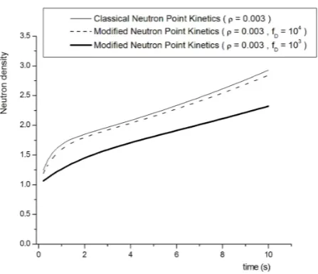
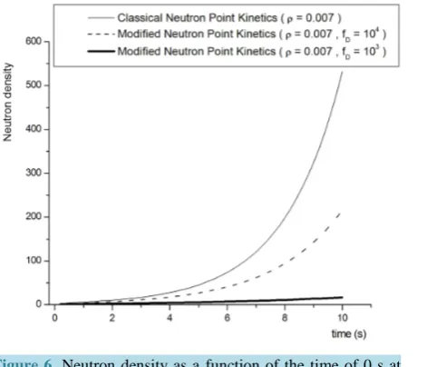
modified point kinetics equation with transport frequency equal to 104 s−1 and modified point kinetics equation with transport frequency equal to 103 s−1. In the first three figures the time interval is from 0 to 100 s and in the last three it goes from 0 to 10 s. Note that in the graph contained inFigure 3 the order of magnitude for neutron density of the classical kinetics and of the modified kinetics are quite different for a reactivity of 0.007.
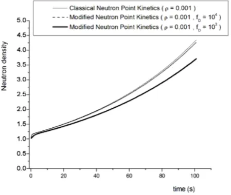
[image:11.595.202.427.336.526.2]The variation in the neutron density as a function of the reactivity is seen through a comparison between the graphs. It is possible to see that, for a reactivity equal to the fraction of neutrons delayed by the total of neutrons, the neutron density obtained by the classical point kinetics equations for a time corresponding to 100 s is of the
[image:11.595.86.538.574.717.2]Figure 1.Neutron density as a function of the time of 0 s at 100 s for a reactivity of 0.001.
Table 1. Parameters used in the tests.
Parameter Symbol Value
Decay constant λ 0.0810958 s−1
Mean generation time Λ 0.002 s
Absorption cross section Σa 0.14 cm−1
Diffusion coefficient D 10 cm
Neutron velocity v 3 × 106 cm/s
Fraction of delayed neutrons β 0.007
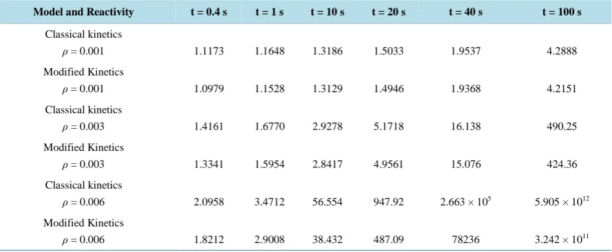
Table 2. Calculation of n(t) (cm−3) with point kinetics for a group of precursors with a neutron transport frequency of 104 s−1.
Model and Reactivity t = 0.4 s t = 1 s t = 10 s t = 20 s t = 40 s t = 100 s
Classical kinetics
ρ = 0.001 1.1173 1.1648 1.3186 1.5033 1.9537 4.2888
Modified Kinetics
ρ = 0.001 1.0979 1.1528 1.3129 1.4946 1.9368 4.2151
Classical kinetics
ρ = 0.003 1.4161 1.6770 2.9278 5.1718 16.138 490.25
Modified Kinetics
ρ = 0.003 1.3341 1.5954 2.8417 4.9561 15.076 424.36
Classical kinetics
ρ = 0.006 2.0958 3.4712 56.554 947.92 2.663 × 10⁵
5.905 × 10¹² Modified Kinetics
ρ = 0.006 1.8212 2.9008 38.432 487.09 78236 3.242 × 10¹¹
Table 3. Calculation of n(t) (cm−3) with point kinetics for a group of precursors with a neutron transport frequency of 103 s−1.
Model and Reactivity t = 0.4 s t = 1 s t = 10 s t = 20 s t = 40 s t = 100 s
Classical kinetics
ρ = 0.001 1.1173 1.1648 1.3186 1.5033 1.9537 4.2888
Modified kinetics
ρ = 0.001 1.0379 1.0798 1.2688 1.4279 1.8083 3.6727
Classical kinetics
ρ = 0.003 1.4161 1.6770 2.9278 5.1718 16.138 490.25
Modified kinetics
ρ = 0.003 1.1185 1.2640 2.3225 3.7127 9.4734 157.38
Classical kinetics
ρ = 0.006 2.0958 3.4712 56.554 947.92 2.663 × 10⁵ 5.905 × 10¹²
Modified kinetics
[image:12.595.88.539.308.706.2]ρ = 0.006 1.2524 1.6157 9.1475 42.311 898.86 8.617 × 10⁶
Figure 3. Neutron density as a function of the time of 0 s at 40 s for a reactivity of 0.006.
Figure 4.Neutron density as a function of the time of 0 s at 10 s for a reactivity of 0.001.
[image:13.595.202.426.501.694.2]Figure 6. Neutron density as a function of the time of 0 s at 10 s for a reactivity of 0.001.
order of 1022, whilst the use of the modified point kinetics equations is of the order of 109, for a neutron trans-port frequency of 103 s−1. Thus, the difference between the results of the models is more significant for high- reactivity situations.
6. Conclusions
The objective of this paper is to obtain a new system of equations called equations of point kinetics modified in which is considered the effect of the time derivative for neutron current density in the Equation (15). In general, the time derivative of the density of neutrons is neglected for the obtainment of the classical model.
The results presented in this article show that the difference between the neutron density obtained from clas-sical point kinetics equations and that obtained from modified point kinetics equations is relevant. With the neu-tron transport frequency equal to 104 s−1 the difference between the neutron density obtained from classical point kinetics equations and that obtained from point kinetics equations without the approximation for the time derivative of neutron current density is relevant. With a neutron transport frequency equal to 103 s−1 the differ-ence between them it is quite significative.
Modified point kinetics equations imply a significant difference in results, in relation to those obtained with the classical point kinetics. Table 1 andTable 2 show that the results from the classical kinetics have an im-portant difference in relation to the model of the modified point kinetics that increases when the frequency is smaller.
References
[1] Duderstadt, J.J. and Hamilton, L.J. (1976) Nuclear Reactor Analysis. John Wiley & Sons Ltd., New York.
[2] Bell, G.I. and Glasstone (1970) Nuclear Reactor Theory. Van Nostrand Reinhold Ltd., New York.
[3] Henry, A.F. (1975) Nuclear Reactor Analysis. The MIT Press, Cambridge and London.
[4] Heizler, S.I. (2010) Asymptotic Telegrapher’s Equation (P1) Approximation for the Transport Equation. Nuclear Science and Engineering, 166, 17-35. http://physics.biu.ac.il/files/physics/shared/staff/u47/nse_166_17.pdf
[5] Espinosa-Paredes, G., Polo-Labarrios, M.A., Espinosa-Martinez, E.G. and del Valle-Gallegos, E. (2011) Fractional Neutron Point Kinetics Equations for Nuclear Reactor Dynamics. Annals of Nuclear Energy, 38, 307-330.
http://www.sciencedirect.com/science/article/pii/S0306454910003816 http://dx.doi.org/10.1016/j.anucene.2010.10.012
[6] Akcasu, Z., Lellouche, G. and Shotkin, L.M. (1971) Mathematical Methods in Nuclear Reactor Dynamics. Academic Press, New York and London.
En-gineering, 90, 40-46. http://www.ans.org/pubs/journals/nse/a_17429 http://dx.doi.org/10.13182/NSE85-7
[8] Zhang, F., Chen, W.Z. and Gui, X.W. (2008) Analytic Method Study of Point-Reactor Kinetic Equation When Cold Start-Up. Annals of Nuclear Energy, 35, 746-749.
http://www.sciencedirect.com/science/article/pii/S0306454907002368 http://dx.doi.org/10.1016/j.anucene.2007.08.015
[9] Hoogenboom, J.E. (1985) The Laplace Transformation of Adjoint Transport Equations. Annals of Nuclear Energy, 12, 151-152. http://www.sciencedirect.com/science/article/pii/030645498590091X
http://dx.doi.org/10.1016/0306-4549(85)90091-X
[10] Fuchs, D. and Tabachnikov, S. (2000) Mathematical Omnibus: Thirty Lectures on Classic Mathematics. American Mathematical Society, Rhode Island.
[11] Hetrick, D.L. (1971) Dynamics of Nuclear Reactor. The University of Chicago Press Ltd., Chicago and London.
[12] Stacey, W.M. (2007) Nuclear Reactor Analysis. 2nd Edition, Wiley-VCH GmbH & CO KGaA, Weinheim.
[13] Kinard, M. and Allen, E.J. (2003) Efficient Numerical Solution of the Point Kinetics Equations in Nuclear Reactor Dynamics. Annals of Nuclear Energy, 31, 1039-1051.
http://www.sciencedirect.com/science/article/pii/S0306454904000027 http://dx.doi.org/10.1016/j.anucene.2003.12.008
[14] Palma, D.A.P., Martinez, A.S. and Gonçalves, A.C. (2009) Analytical Solution of Point Kinetics Equations for Linear Reactivity Variation. Annals of Nuclear Energy, 36, 1469-1471.
http://www.sciencedirect.com/science/article/pii/S0306454909001947 http://dx.doi.org/10.1016/j.anucene.2009.06.016