Application of Ford-Fulkerson Algorithm to Maximum Flow in Water Distribution Pipeline Network

Application of Ford-Fulkerson Algorithm to Maximum

Flow in Water Distribution Pipeline Network

Myint Than Kyi*, Lin Lin Naing**

*Department of Engineering Mathematics, Technological University (Mandalay). Mandalay Division, Myanmar. **Faculty of Computing, University of Computer Studies, Hinthada, Ayeyarwady Division, Myanmar

DOI: 10.29322/IJSRP.8.12.2018.p8441

http://dx.doi.org/10.29322/IJSRP.8.12.2018.p8441

Abstract- In this paper, well known Ford-Fulkerson algorithm in graph theory is used to calculate the maximum flow in water distribution pipeline network. The maximum flow problem is one of the most fundamental problems in network flow theory and has been investigated extensively. The Ford-Fulkerson algorithm is a simple algorithm to solve the maximum flow problem and based on the idea of searching augmenting path from a started source node to a target sink node. It is one of the most widely used algorithms in optimization of flow networks and various computer applications. The implementations for the detail steps of algorithm will be illustrated by considering the maximum flow of proposed water distribution pipeline network in Pyigyitagon Township, Mandalay, Myanmar as a case study. The goal of this paper is to find the maximum possible flow from the source node s to the target node t through a given proposed pipeline network.

Index Terms- Flow network, Ford-Fulkerson algorithm, Graph Theory, Maximum flow, Water distribution network.

I. INTRODUCTION

n many fields of applications, graphs theory [1] plays vital role for various modelling problems in real world such as travelling, transportation, traffic control, communications, and various computer applications and so on [2]. Graph is a mathematical representation of a network and it describes the relationship among a finite number of points connected by lines. The maximum flow problem is a type of network optimization problem in the flow graph theory [3]. A flow network is a directed graph where each edge has a capacity and receives a flow as weighted values. A flow must satisfy the restriction that the amount of flow into a node equals the amount of flow out of it except source node, which has only outgoing flow, and sink node, which has only incoming flow [4]. In practice, the flow problems can be seen in finding the maximum flows of currents in an electrical circuit, water in pipes, cars on roads, people in a public transportation system, goods from a producer to consumers, and traffic in a computer network, and so on.

II. RESOURCES AND METHOD

A simple, connected, weighted, digraph G is called a transport network if the weighted value associated with every directed

edge in G is a non-negative number. This number represents the capacity of the edge and it is denoted by 𝑐_𝑖𝑗 for the directed edge from node 𝑖 to node 𝑗 in G [5]. We consider a network of pipelines of water distribution system and the case of network of pipes having values allowing flows only in one direction. This type of network is represented by weighted connected digraph in which District Metered Areas (DMA) are represented by vertices and lines which given water flows through by edges and capacities by weights. To provide the maximum flow from source vertex to sink vertex is one of the most important things in all transmission network. Source vertex is produced flows along the edges of the digraph G and sink vertex is received [1]. The residual graph can be defined by providing a systematic way in order to find the maximum flow. The residual capacity of an edge can be obtained by using the formula 𝑐𝑓_𝑖𝑗= 𝑐_𝑖𝑗− 𝑓_𝑖𝑗 and a residual network can be defined by giving the amount of available capacity.

A. Problem Definition

The maximum flow problems involve finding a possible maximum flow through a single-source to single-sink flow network. The maximum flow problem can be seen as a special case of more complex network flow problems, such as the circulation problem [6]. The problem is given by a directed graph G with a start node s and an end node t. Each edge has associated with it a positive number called its capacity. A flow in a network is a collection of chain flows which has the property that the sum of the number of all chain flows that contain any edge is no greater than the capacity of that edge [7]. The goal is to provide as much flow as possible from s to t in the graph. The flow in any edge is never exceeded its capacity, and for any vertex except for s and t, the flow in to the vertex must equal the flow out from the vertex. On any edge we have 0 ≤ 𝑓_𝑖𝑗≤ 𝑐_𝑖𝑗. This is called capacity constraint or edge condition. As a flow constraint, flow into vertex is equal to flow out of vertex for any vertex. In a formula,

� 𝑓𝑘𝑖 𝑘

− � 𝑓𝑖𝑗 𝑗

= � 0 if vertex 𝑖 ≠ 𝑠, 𝑖 ≠ 𝑡−𝑓 at the source node 𝑓 at the target (sink)𝑡, inflow − outflow

where 𝑓 is the total flow. Subject to these constraints, the total flow into target node t can be maximized.

B. Ford-Fulkerson Algorithm for maximum flow

In 1955, Ford, L. R. Jr. and Fulkerson, D. R. created the Ford-Fulkerson Algorithm [7]. This algorithm starts from the initial flow and recursively constructs a sequence of flow of increasing value and terminates with a maximum flow [8]. The idea behind the algorithm is simple. We send flow along one of the paths from source to sink in a graph with available capacity on all edges in the path that is called an augmenting path and then we find another path, and so on [6].

1). Notation and Steps of the Algorithm

For every edge connected from node 𝑖 to node 𝑗, we use the notation (𝑖, 𝑗):

∆𝑖𝑗= 𝑐𝑖𝑗− 𝑓𝑖𝑗 for forward edges ∆𝑖𝑗= 𝑓𝑖𝑗 for backward edges

∆= min ∆𝑖𝑗 taken over all edges of a path.

The Ford-Fulkerson algorithm has two main steps. The first step is a labelling process that searches for a flow augmenting path and the second step is to change the flow accordingly. Otherwise, no augmenting path exists, and then we get the maximum flow [4]. The detail steps of the algorithm are stated as follows [1]:

Step 1. Assign an initial flow 𝑓_𝑖𝑗 (or may be given), compute f.

Step 2. Label s by ∅. Mark the other vertices “unlabelled.” Step 3. Find a labelled vertex i that has not yet been scanned.

Scan i as follows. For every unlabelled adjacent vertex j, if 𝑐𝑖𝑗> 𝑓𝑖𝑗 compute

∆𝑖𝑗= 𝑐𝑖𝑗− 𝑓𝑖𝑗

and ∆𝑗= �_min(∆∆𝑖𝑗 𝑖𝑓 𝑖 = 1 𝑖, ∆𝑖𝑗) 𝑖𝑓 𝑖 > 1

and label j with a “forward label” (𝑖+, ∆_𝑗)or if 𝑓_𝑖𝑗> 0, compute ∆_𝑗= min�∆_𝑖, 𝑓_𝑗𝑖� and label j by a “backward label” (𝑖−, ∆_𝑗).

If no such j exists then OUTPUT f . Stop. Else continue (i.e., go to step 4).

Step 4. Repeat Step 3 until t is reached.

[This gives a flow augmenting path 𝑃: 𝑠 → 𝑡.]

If it is impossible to reach t, then OUTPUT ƒ. Stop. Else continue (i.e., go to Step 5).

Step 5. Backtrack the path P, using the labels.

Step 6. Using P, augment the existing flow by∆_𝑡. Set 𝑓 = 𝑓 + ∆𝑡

Step 7. Remove all labels from vertices 2, … , 𝑛. Go to Step 3.

This is the end of the algorithm. The flowchart illustrating for the maximum flow of water distribution network is as follow:

Fig. 1 Flowchart for maximum flow of water distribution network III. RESULTS AND DISCUSSION

In this paper, the application of graph theory to find the maximum flow of water distribution network has been illustrated by using the Ford-Fulkerson algorithm [1] to the proposed water distribution pipeline network of Pyigyitagon Township in Mandalay, Myanmar. One who wants to know the possible maximum flow required the detail implementation of this algorithm. The weights on the links are referred as capacities and current flows for corresponding edges.

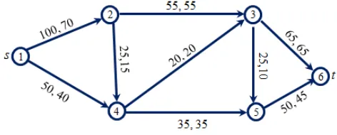
The flow network of pipeline is a directed graph with two distinguished nodes; source and sink. Since the sizes of pipes used in this network may not be the same, the capacity for each pipe may also be different. So it can only maintain a flow of a certain amount of water. Anywhere those pipes meet, the total amount of water coming into that junction must be equal to the amount going out. Each edge between two nodes has a non-negative capacity 𝑐 and receives a flow 𝑓 where amount of flow on an edge cannot exceed its capacity [3]. The first number on each edge represents capacity and the second number represents current flow (liter/sec). In this pipeline network, we denote the source node 1 as “s” and the sink (target) node 6 as “t” as shown in Fig. 3.

Fig. 3 Representation of digraph for proposed network of water pipeline in Pyigyitagon Township, Mandalay, Myanmar

A. Implementation of the Algorithm

The implementation of the Ford-Fulkerson algorithm is illustrated to find the maximum flow for proposed water distribution pipeline network in Pyigyitagon Twonship, Mandalay from source node s to sink node t. We can choose any path from source to sink for each iteration step as an augmenting path by using the edge with the non-zero residual capacity in previous step. This means that the edge with maximum flow cannot be used as a segment of augmenting path.

The detail implementation of algorithm can be seen as follows:

Step 1 An initial flow 𝑓 = 50 + 20 = 70(Given).

Step 2 Label (𝑠 = 1) by ∅. Mark 2, 3, 4, 5, 6 “unlabelled”

Step 3 Scan 1

Compute ∆₁₂= 100 − 50 = 50 = ∆₂. Label 2 by (1+_{, 50).}

Compute ∆₁₄= 50 − 20 = 30 = ∆₄. Label 4 by (1+, 30).

Step 4 Scan 2.

Compute∆₂₃= 55 − 40 = 15, ∆₃= min(∆₂, ∆₂₃) ∆3= min(50, 15) = 1. Label 3 by (2+, 15). Scan 3.

Compute∆₃₆= 65 − 45 = 20, ∆₆= min(∆₃, ∆₃₆) ∆6= min(15, 20) = 15. Label 6 by (3+, 15). Step 5 𝑃: 𝑠 = 1 → 2 → 3 → 6 = 𝑡 is a flow augmenting path.

Step 6. ∆_𝑡= 15. Augmentation gives 𝑓₁₂= 65, 𝑓23= 55,𝑓36= 60.

Augmented flow 𝑓 = 70 + 15 = 85.

Step 7 Remove labels on vertices 2 … , 6. Go to Step 3.

Fig. 4 Flow augmenting path 1-2-3-6 Step 3 Scan 1

Compute ∆₁₂= 100 − 65 = 35 = ∆₂. Label 2 by (1+, 35)

Compute ∆₁₄= 50 − 20 = 30 = ∆₄. Label 4 by (1+, 30)

Step 4 Scan 2.

Compute ∆₂₄= 25 − 10 = 15, ∆₄= min(∆₂, ∆₂₄). ∆4= min(35, 15) = 15. Label 4 by (2+, 15). Scan 4.

Compute ∆₄₃= 20 − 15 = 5, ∆₃= min(∆₄, ∆₄₃) ∆3= min(15, 5) = 5. Label 3 by (4+, 5). Scan 3.

Compute ∆₃₆= 65 − 60 = 5, ∆₆= min(∆₃, ∆₃₆). ∆6= min(5, 5) = 5. Label 6 by (3+, 5).

Step 5 𝑃: 𝑠 = 1 → 2 → 4 → 3 → 6 = 𝑡 is a flow augmenting path.

Step 6 ∆_𝑡= 5. Augmentation gives 𝑓₁₂= 70, 𝑓₂₄= 15, 𝑓43= 20, 𝑓36= 65.

Augmented flow 𝑓 = 85 + 5 = 90.

Step 7 Remove labels on vertices 2 … , 6. Go to Step 3.

Fig. 5 Flow augmenting path 1-2-4-3-6 Step 3 Scan 1

Compute ∆₁₄= 50 − 20 = 30 = ∆₄. Label 4 by (1+, 30).

Step 4 Scan 4.

Compute ∆₄₅= 35 − 15 = 20, ∆₅= min(∆₄, ∆₄₅). ∆5= min(30, 20) = 20. Label 5 by (4+, 20). Scan 5.

∆6= min(20, 25) = 20. Label 6 by (5+, 20). Step 5 𝑃: 𝑠 = 1 → 4 → 5 → 6 = 𝑡 is a flow augmenting path.

Step 6 ∆_𝑡= 20. Augmentation gives 𝑓₁₄= 40, 𝑓₄₅= 35, 𝑓56= 45.

Augmented flow 𝑓 = 90 + 20 = 110.

Fig. 6 Flow augmenting path 1-4-5-6

Finally, there are no augmenting paths possible from s to t, and then the flow is maximum flow. The maximum flows for all pipelines in network have been calculated by iteration process of Ford-Fulkerson algorithm and can be seen in Fig. 7.

Fig. 7 Maximum flows in pipeline network from source node s to sink node t

The maximum flow will be the total flow out of source node which is also equal to total flow in to the sink node. In this case, total flow out from source node s is 70 + 40 = 110 and total flow in to the sink node t is 65 + 45 = 110 and hence maximum possible flow for this network is 110 liters/sec.

B. Comparison and Recommendation

The maximum flow problem has been studied by many researchers because of its importance for many areas of applications [3]. There are many algorithms to find the maximum flow problems, among them the most popular algorithms are Ford-Fulkerson algorithm, Edmonds-Karp algorithm, and Goldberg-Tarjan algorithm. Ford-Fulkerson uses depth-first-searches to find augmenting paths through a residual graph, while Edmond-Karp uses breath-first-searches to achieve a polynomial time complexity, and Goldberg-Tarjan solves the problem by gradually pushing flow through the residual graph. Although they all are algorithms to find maximum flow, the special features of them are different. Ford-Fulkerson algorithm can be applied to find the maximum flow between single source and single sink in a graph, while Edmonds-Karp algorithm and Goldberg-Tarjan algorithm use breath-first-searches and are performed from the sink, labelling each vertex with the distance to the sink [10]. All the works above and some other works gave algorithms that have good computational performance. But the algorithms in these works are very complicated and some of them are only suitable for the flow networks with specific

structure [6]. The comparison for calculation times can be checked in the following table [4].

TABLE I

COMPARISON FOR TIME COMPLEXITY OF MAXIMUM FLOW ALGORITHMS

Maximum-flow Algorithm Time Complexity*

Ford-Fulkerson 𝑂(𝑛𝑚 𝑐)

Edmonds-Karp 𝑂(𝑛𝑚2) Goldberg-Tarjan _{𝑂 �𝑚𝑛 log �}𝑛

2

𝑚��

* n, m and c are number of nodes, edges and capacities respectively.

Although the calculation time for Ford-Fulkerson algorithm is higher than other algorithms, it is simple to implement in finding the maximum flow. The Edmonds-Karp algorithm is a small variation on the Ford-Fulkerson algorithm. Goldberg and Tarjan algorithm manipulates the preflow rather than an actual flow in a graph. Other modified algorithms are developed to reduce computation time [3], [6], but these algorithms are complicated and required high speed processors such as supercomputer to simulate the problem with 1000 nodes and over 94000 arcs and run for optimal flow [6]. The Ford–Fulkerson algorithm is guaranteed to terminate if the edge capacities are nonnegative real values. For these reasons and above comparison, we strongly recommend that Ford-Fulkerson algorithm is an algorithm to get the solution for finding maximum flow with simple procedure.

IV. CONCLUSION AND FUTURE WORKS

In this paper, Ford-Fulkerson algorithm in flow graph theory has been implemented to find the maximum possible flow in water distribution pipeline network of Pyigyitagon Township, Mandalay, Myanmar. The main idea of the algorithm is to find a path through the graph from the source to the sink, in order to send a flow through this path without exceeding its capacity. Then we find another path, and so on. A path with available capacity is called an augmenting path. Maximum flow for proposed water distribution pipeline network has been developed to implement the algorithm. Actually, the flow rate of water in pipeline is depending upon the size of used pipes and pressure at each node. But we have considered only capacity and flow rate of water in the network and other factors such as size of pipes and pressure at each node are not considered in this paper.

As the future works, this algorithm can also be used to model traffic in a road system, fluids in pipes, currents in an electrical circuit, or anything similar in which something travels through a network of nodes. Moreover, based on the flowchart and detail calculation procedure, one can create computer codes such as C/C++, or JAVA, running these codes by using nonnegative real weighted values from actual information and data to solve general Ford-Fulkerson maximum flow problems.

ACKNOWLEDGMENT

Naing, Professor and Head, Faculty of Computing, University of Computer Studies, Hinthada, for his invaluable comments and perfect supervision throughout my research. Her special thanks are due to U Myo Thant, Head of Water and Sanitation Department, Mandalay City Development Committee, Mandalay, Myanmar for his supports to get required data and information to her research. Finally, the author’s thanks are to her beloved mother, brothers and sister because her research cannot be done successfully unless they support it.

REFERENCES

[1] Erwin Kreyszig, Advanced Engineering Mathematics, 10th edition. Copyright © 2011 John Wiley & Sons, Inc. All rights reserved.

[2] Meysam Effati, Analysis of Uncertainty Considerations in Path Finding Applications [Online] Available: http://5thsastech.khi. ac.ir/data1/ civil/1%20%2812%29.pdf.

[3] Ola M. Surakhi, Mohammad Qatawneh, Hussein A. al Ofeishat, “A Parallel Genetic Algorithm for Maximum Flow Problem,” (IJACSA) International Journal of Advanced Computer Science and Applications, Vol. 8, No. 6, 2017. [Online] Available: http://thesai.org /Downloads/Volume8No6/Paper_20-A_Parallel_Genetic _Algorithm_ for_Maximum.pdf.

[4] Flow network [Online] Available: https://en.wikipedia.org/ wiki/ Flow_network#Augmenting_paths.

[5] Santanu Saha Ray, GraphTheory with Algorithms and its Applications In Applied Science and Technology, Copyright Springer India. 2013. ISBN 978-81-322-0750-4.

[6] Zhipeng Jiang1, Xiaodong Hu1, and Suixiang Gao. “A Parallel Ford-Fulkerson Algorithm For Maximum Flow Problem”. Chinese Academy of Sciences, Beijing, China.

[7] L. R. Ford, JR. and D.R. Fulkerson, “Maximal Flow Through a Network”. Rand Corporation, Santi Monica, California. September 20, 1955. [8] M. Shokry, “New Operators on Ford-Fulkerson Algorithm”. IOSR Journal

of Mathematics (IOSR-JM). Vol. 11, Issue 2. Mar-Apr. 2015. pp. 58-67. [9] Tun Win U, “Proposed Water Supply Master Plan and Existing

Wastewater Management System in Mandalay Industrial Hub”. Mandalay City Development Committee. 2016.

[10] Markus Josefsson, Martin Mützell, “Max Flow Algorithms, Comparison in regards to practical running time on different types of randomized flow networks”. Degree Project in Computer Science, DD143X. Sweden, Stockholm 2015.

AUTHORS

First Author – Myint Than Kyi, Lecturer, Department of

Engineering Mathematics, Technological University (Mandalay). Mandalay Division, Myanmar.

Email address: [email protected]

Second Author – Dr. Lin Lin Naing, Professor and Head,

Faculty of Computing, University of Computer Studies, Hinthada, Ayeyarwady Division, Myanmar.