Computer vision assistant for train rolling stock examination (RSE) using level set models

(1)

COMPUTER VISION ASSISTANT FOR TRAIN ROLLING STOCK

EXAMINATION USING LEVEL SET MODELS

Krishnamohan Kaja, Ch. Raghava Prasad and M.V.D. Prasad

Department of Electronics and Communications Engineering, Koneru Lakshmaiah Education Foundation, Green Fields, Vaddeswaram, Guntur DT, Andhra Pradesh, India

E-Mail: [email protected]

ABSTRACT

Rolling stock Examination (RSE) is automated with computer vision sensors and programming models in development of a fully automated ARSE model to assist human examiners. Four algorithms are being tested in this work. We start with Chan Vese Level Sets (CV_LS); Morphological Differential Gradient based Level Sets (MDG-LS), which are global segmentation models. In the next part, we propose shape prior level sets (SP_LS) and Invariance Shape Prior Level Sets (ISP_LS), which are local segmentation methods. This work compares these proposed models in the aspects of segmentation quality to correctly identify a bogie part and to extract a defective part. Structural Similarity Index (SSIM) is the measure to correctly identify a bogie part. Image Quality Index (IQI) measures quality of segmented bogie part form all the 4 algorithms. Peak signal to noise ratio (PSNR) tests the ability of the proposed algorithms to identify defects in the bogie parts. ISP_LS is the best local segmentation algorithm for both bogie part detection and defect identification on rolling stock visual information at 4 different times of the day.

Keywords: rolling stock examination, level sets, shape priors, performance analysis, high speed video segmentation.

1. INTRODUCTION

Rolling stock examination (RSE) is manual checking of bogie parts, when train is moving at 30KMPH to identify accident causing defects. Here manual checking involves a team of 3 humans putting their eyes, ears and intelligence to the limits. Figures 1 and 2 shows the 3D view and 2D line diagram of the two different bogies currently used in Indian Railways. The system operates on all passenger trains at every train station across Indian subcontinent. This saves trains from accidents while moving at high speeds. This work proposes to replace trained human eyes with high speed cameras and intelligence with processing algorithms.

High speed (HS) cameras with a frame rate of 240fps are used to capture moving bogie videos under different ambient lighting environments. Various algorithms related to segmentation are proposed by us in the past for segmenting the bogie parts for defect identification [1, 2]. Six highly trained men save a train for derailment using the power of concentration during RSE. Even though Indian Railways has a full proof system using highly trained humans for RSE, the system suffers from human mistakes due to environmental factors, workload and shifting focus on long trains. The identified defects are passed to the maintenance staff only in the next station. The current manual RSE model puts a huge financial burden on the system.

Figure-1. Train under carriage model: FIAT Bogie.

By replacing human eyes with high speed cameras for capturing trains moving at 30KMPH with motion blur, which makes identification of closely packed bogie parts impossible. The best model for extracting individual parts in closely packed images is snakes [3-6]. Active contours are the most researched convex segmentation algorithms on complex natural images [7-13]. Hence, this work focus on testing 4 level sets for RS Video frame segmentation.

There is an increase an increase in computer vision based algorithms for human safety monitoring during transit. But most of the research is on waterways, airways and roadways. Train rolling stock is one area that significantly dominates railway passenger safety which is monitored by humans 24 hours across the world.

(2)

Indian Railways Invention as shown in Figure-2. Figure-3 shows the manual procedure followed for rolling stock examination.

Figure-2. Train under carriage: ICF Bogie.

Figure-3. Showing manual rolling examination in progress.

Figure-4 shows the recording of rolling stock near to a railway station on Indian subcontinent. Using a high speed 240fps action camera, a RS video dataset of 20

trains is created at 4 different times of the day. For this work, only ICF rakes are recorded.

Figure-4. Rolling stock data collection with high speed action camera recording at 240fps.

2. LITERATURE REVIEW

Computer vision research is currently driving most of the software industry giants such as Google and Facebook. Research shows face recognition; image search; video compression and playback; deep learning algorithms are revenue generators for the tech sector companies. Vision research has deeply made inroads into automobile with autonomous driving cars [14], transportation monitoring [15], structural quality assessment[16], agricultural [17] and manufacturing [18] industry from last decade onwards. Specialized cameras such as high speed,

laser and hyperspectral cameras are being used for video capture for monitoring and testing applications.

Narayanaswami, et al [19] provides a vision for future of transportation in urban environments. The ideas discussed in this work help understand the link between technology and automation required to save on time and finances with focus on avoiding accidents. In [20], Sabato,

et al uses 3D digital image correlation (DIC) algorithms to inspect railroad ties and ballast. Two cameras at a specific displacement are mounted on a rail car moving at 60Kmph to produce a 3D image. Deformation of railway tracks is identified with 3D DIC and pattern projection algorithms.

SECONDARY SUSPENSION

SAFETY STRAP

LOWER SPRING BEAM PRIMARY SUSPENSION

VERTICAL SHOCK ABSORBER

(3)

US Federal Railroad Administration data between the years 2005 and 2015 show 16000 derailment due to track, ballast and rolling stock failure.

Automation of Rolling stock is important for railways around the world for cutting costs and saving trains from derailment. Computer vision processing can be used for monitoring rolling stock to identify defects in bogies. Hart, et al [21] used multispectral imaging to extract bogie segments for inspection. They recorded both RGB videos and thermal videos of a moving train with processed the frames using panoramic representation and correlation. The focus was on detecting high temperature regions on the undercarriage parts such as brake shoes, axel box, air conditioning blowers and wheel joints. However, the work is of great use to rail companies with a shortcoming in frame rate as the cameras induce blurring which makes it difficult to identify non-heating parts on the moving train.

Kim, et al [22] transforms the rolling stock brake inspection problem into image curve fitting problem. The methods developed use a database setting of the undercarriage of the train bogies and use cure fitting tools to identify brake alignments during train movement. The cost of the setup poses a big drawback for such a system to be implemented in real time. The patent from Sanchez-Revuelta, et al [23], shows the use of computer vision for rolling stock examination two decades prior to our work. This patent says artificial vision will be used to monitor rolling stock by mounting cameras on the train. The captured videos on a moving train call for many fold misalignments and more computation power is required to again process the same for a closer inspection.

Kazanskiy, et al [24], proposed a vision based computer technology for rolling stock monitoring system. The work integrates glare free lighting system, video compression models and structured lighting module to detect the presence of train on tracks to monitor rolling stock. This work reaches close to making rolling stock a reality, however there is little mention on evaluating each bogie part for inspection. Freid, et al [25] provides an undercarriage arrangement with lighting and a camera for rolling stock evaluation and processing. They used simple edge detection models for extracting axle rod and measuring its temperature using thermal camera. The model provides a good insight into the importance of the problem in automating rolling stock examination. In [26] and [27], the authors proposed a 3D reconstruction for monitoring contact strips and rolling stock wheel surfaces. These methods are effective as the 3D models perfectly reconstruct the surface defects in moving parts. These methods use lot of computation time and energy for processing as it is difficult to model all defective surfaces. With all these gaps in rolling stock automation using computer vision, we propose a high-speed sensor to capture moving trains and advanced state of the art level sets formulations to identify bogie parts and defective bogie parts. The camera sensor records at 240fps in wide angle mode covering the entire bogie in one frame as shown in figure 10 with a resolution of 640×480 pixels. The bogie parts segmentation is formulated as a convex

curve fitting problem with pre-information regarding the shape of the bogie part. Four different level sets are tested in this work, which are a part of our previous segmentation modules [1]. Here the algorithms are tested for perfect and defective bogie parts with SSIM [28, 29], IQI [28] and PSNR [28].

From the Indian railway manual (http://www.intlrailsafety.com/capetown/3_024_amitabh.d oc), there are around 10 important and crucial things to be checked during rolling examination. This paper reports the simulations for extracting and identifying bogie parts as defective and non-defective based on the quality of the algorithms used.

The rest of the paper is organized as: section 3 describes the different Active Contour Level Sets. Results and discussion with various train models and defects is presented in section 4 with conclusions in section 5.

3. LEVEL SETS SEGMENTATION ON HS VIDEO FRAMES

3.1 Generalize level sets (G_LS)

Active Contour models first introduced by Terzopoulos [30] to modelling shape by using segmented images. Evolution of equation in the active contour is labelled snake principally was familiarized by Kass [31]. Let _{: AC} 2

XY

F   be observable and controlled by a set of positive real numbers in a space holding 2D shapes. The subspace target is_{S : AC}__R2_{, here}_S_F_{is a subset of} image. The energy function of active segmentation:

1

0{ ( ( )) ( ( ))}

XY F

S I

E 



E V s E V s ds (1)

Here the snake energy is S

E . The snake’s internal energy is I

E and the image energy is_EFXY . Where

the snake is positioned on the image frame at:

( ) ( ( ), ( ))

V s  X s Y s

(2)

and the internal energy I

E in the snake describes its twisting on the image and the _EFXY image forces push the

snake onto image boundaries in the deformable curve. The

I

E is defined as:

2 2

( ( ) ( ) ( ) ( ) ) 2

I s s s s

E     

(3)

Where( )s is the first order derivation of ( )s

which tracks curve length variations and ( )s provides degree of tightening in all directions. Correspondingly,

( )s

(4)

2 ( , )

xy F

E   F x y (4)

3.2 Chan Vese level sets (CV_LS)

The Chan Vese Level Setsin [32] is arithmetically expressed by minimizing energy function defined by:



,



min ( , )

chan vese I I chan vese

E E



    

(5)

Here the initial contour is and the resulting contour shape _I_{is to be discovered. The object borders}

in an image are discovered by the initial contour 2

: C

F   to( )I

and _( )E _{regions as contour interior}

and exterior to



. The energy function of the Chan Vese Level Sets is minimized by using Mumford-shah [33] piece wise linear function.

The equation of the minimization function defined as:



_{( )}



2



_{( )}



2

1 2

1 1

( , ) ( , )

2 I 2 E

chan vese I E

E



ds



F x y dxdy F x y dxdy

                 





(6)

In this above equation, the initial term points to the arc length



1



min( , )

arg



l( )  

  , which provides the

consistency ofthroughout the curve evolution and

l

( )



is contour perimeter. The next term in equation 6 is a combination of integrals. The first integral force pushes the contour to the image objects and next integral guarantees the differentiability of the contour . The integral is evaluated on the internal and external contour regions defined by _I and _E_{respectively.}

In Equation 6 the weights are positive real numbers

  

1

,

2

0

. The Chan Vese level set is formulated using Mumford-shah distance function as:





2

1 2

internal( )

( , ) ( , )

chan vese

E



ds



F x y x y dxdy

 









 

(7)

The Chan Vese level sets model considers area of pixels inside and outside of the contour given by.





( )

, ( , )lies inside 1

( , )

,

, ( , )lies outside 1 ( , ) I E I I E E where x y

F x y dxdy

x y

where x y

F x y dxdy

     _{ }  _            



(8)

Chan Vese Level Sets model evaluates and finds the values of , on the image

F x y

( , )

with the energy model defined as

 



_{( )}



2



_{( )}



2

1 2

1 1

, ( , ) ( , )

2 2

I I E

chan vese I E

E



ds



x y dxdy



F x y dxdy F x y dxdy

                    





(9)

The initial two relations provide regularization for length and area of the contour to control its size using the parameters



1



0,



2



0 and





0

. The next two terms make the model



 

x y

,

adjust to the

I x y

( , )

. The

above equation 9 to create a global minimizing problem in image segmentation.

By using the level set models in [34] to solve the minimizing problems in equation 9 and the modified equation of the level set function as

 

() ()

( ) () ( ) 2

2

, ,

( ) 2

1

( , , ) min ( ( , ) ) ( , )

( ( , ) ) (1 ( , ) ) ( ( , )) I E

chan vese I E I

E

I

E

E F x y x y

F x y x y dxdy  x y dxdy



                          





(10)

Here Heaviside function is

 

( )

. The level set in equation.10 is updated iteratively by minimizing the

gradient descent model defined as to arrive a minimum value for( , )x y :

( ) 2 ( ) 2

1

( , ) ( )(( ( , ) ) ( ( , ) ) .

( , )

t I E x y

F x y F x y

x y

  

          

(5)

Here the pixel locations in the image are denoted as x and y. the delta function is

 

( )

and iterative adaptations are initiated using the equations of _( )I

and

( )E

 as

( )

( , ) ( ( , ))

( ( , ))

I

F x y x y dxdy

x y dxdy

       



(12) ( )

( , )(1 ( ( , )))

(1 ( ( , )))

E

F x y x y dxdy

x y dxdy

         



(13)

Figure-5(a) shows the full segmentation of the rolling frames using the Chan Vese Level Sets Model. The resolution of the video frame is 760×1080 and the CV_LS takes around 750 iterations for achieving the desired segmentation. The next method is used to improve the speed and segmentation accuracy of ultrasound medical images [28]is being tested for rolling stock segmentation.

3.3 Differential gradient based level sets (MDG-LS) The previous Chan Vese level set algorithm uses image gradients to detect object regions. Image gradients are prone to rapid brightness variations as can be found in the rolling stock video frames. Due to brightness inconsistency the contour spread takes in large iterations as pointed out in[35]. The challenging task for rolling stock frame segmentation is in decreasing the computation time with optimal bogie segmentations for quick maintenance.

The Chan Vese technique is a capable model for many segmentation problems, we proposed to replace the Chan Vese model’s image gradient in equation (11) with a Morphological Differential Gradient (MDG) term. A video frame xy_: 2

F D  in space D, we apply dilation and

erosion morphological operators on the grey scale rolling frame with a line structuring mask having m rows and n Columns mn

:

2

, ,

{

,...., }

L

D

 

m n

 

M

defined as

,

{max( | , to }

xy xy mn x m y n mn

d

F F L  F   l m n N N (14)

,

{min( | , to }

xy xy mn x m y n mn

e

F F



L  F   l m n N N (15)

Here mn

L represents line structuring element of size M. Four different line angles

{ / 4, / 2, 3 / 4, }



with single region overlapping pixels’ are used to create the structuring element mn

L . In dilation _d_{and in erosion} e

 are morphological gradient operators respectively. In

equation 11, .

xy xy O O  

 is replaced with MGD term as

 

.

 

.

d xy e xy

d e

d xy e xy

O O

 _ 

 _  _ . This minor changes in

image energy is visibly noticeable in Figure-5(b).

As shown in Figures 5(a) and (b) the arrows point to the locations where there is a considerable change in segmentation accuracy between CV_LS and MDG_LS. During experimentation it was noticeable that MDG_LSis 44% faster than CV_LS model for rolling stock segmentation.

Figure-5. (a) Segmentation with CV_LS Model [32] (b) segmentation with MDG_LS[36].

In the above two methods identification and extraction of each bogie for checking is difficult. Even though the regional segmentation improved in quality and speed, the model is still not suitable for vision based rolling examination. The following two techniques use shape priors and shape invariance of each bogie part for extraction and defect identification at a faster rate.

3.4 Shape prior level sets (SP_LS)

Adding to existing Chan Vese (CV)[37] level set in equation 10 is the shape prior model proposed in [38] producing an energy function characterized as

( ) ( ) ( ) ( )

( , , ) ( , , )

chan vese shape chan vese I E Shape I E

S S

E  E    E    (16)

Form equation 10 the primary term represents the data term from Chan Vese level set in equation 16 and the later shape prior energy function is defined as

 







 







2

( ) ( )

( , , ) , ,

Shape I E

S S S

E x y x y dxdy



(6)

Figure-6. Curve evolution in SP_LS.

Here the shape prior term



S



x y,



is dependent on the position of objects in the image. The energy term for multiple shape priors is

  _ _

 

2

( ) 2

,

( ) 2

1 1 log

S j

d N chan vese shape n

j

E e

N

      

 

 

  



 

 

  _ _





 (18)

For using equation.18, the number of shape priors should be limited and apprehending the statistical shape from a few different shapes is a difficult task. Hence, we preferred single object extraction with single shape prior by simulating equation 16. The shape prior level set evolution on a frame of rolling stock is shown in figure 6. In this figure the shape prior is fixed for this specific frame of the bogie. The position of the shape changes will affect the segmentation outputs.

3.5 Invariance shape prior level sets (ISP_LS)

The previous SP_LS focuses on a bogie part for segmentation resulting in good quality bogie parts for classification. However, the initial contour must be manually shifted to the bogie interest part for extraction making the process time consuming and precision oriented. The solution in [39] introduces a signed distance function for shape encoded level sets making the

segmentation process independent of object positions, orientations and scales in the images. To create a unique connection between its adjacent level set and a

pre-defined shape model



Shape, it will be assumed that

0, inside

Shape







,





0, outside



Shapeand

 

1

everywhere else. There are many ways to define this signed distance function [40, 41], out of which we use the most commonly used with constrains towards rotation, scaling and translational properties. In this work we propose to use  as the initial contour and



Shape is the shape prior contour to compute level set area difference as in [42].







 





 



2

, Shape Shape

d

 

H



x H



x dx





_

 (19)

In this work, around 20,000 frames of a train are used to identify parts with only one shape prior of a bogie part. As the train moves either to the left side of the frame or to the right side of the frame, the bogie has a side movement in only x-direction. The shape invariance of the shape prior is handled by

 







 







2

0, 0

Shape Shape Shape

E



d

 

H



x H



s x t_ _ dx



  

_

  (20)

Here the shape scale and translational values are represented with

s

and

t

. Local energy minimization

between



0,



Shape

  , maximizes the possibility of finding precise shape in the densely-packed bogie objects in the rolling stock frame. The curve evolution expression is obtained by applying Euler-Lagrange equation on (20),

 





 



0

0 0

2 Shape

H H

t



_{ }

_

_

 _ _ _

 (21)

(7)

term and equation 10 CV level set function produces a total level set energy function defined by

(1

)

T C Shape

E





E

 



E

(22)

Here shape prior energy on the image is controlled by . We develop segmentation model for single shape priors with the energy functional used from evolution equations in equation (10) and equation (21) as

 



 

2



2









 



. ( ) ( ) 2 1 Shape

I x C I x C H H

t



_{  }



_

_

_



 

 

 _ _ _ _ _ _ _ _ _ _

    

 __ _ _ __ _ (23)

Were Cand Care updated iteratively using

the expressions in equation.13. The curve evolution of shape invariance level set is as shown in Figure-7. The shape prior model is specified as red contour and

transformed shape prior is showed as yellow contour. The green contour evolve son the frames for finding the bogie parts.

Figure-7. Curve evolution in ISP_LS model.

4. RESULTS AND DISCUSSIONS

The above discussed 4 models are extensively tested for accuracy and speed of segmentation methods on 10 different bogie parts on a train moving at 30KMPH. A high-speed camera captures the transit bogies at 240fps to evade motion blur. The camera is additionally equipped with a wide-angle capture lens to record the whole bogie in one frame as shown within the Figure-8. Four completely different trains having similar configuration and recorded parts at different time variations for experimentation. These trains in Asian Country (India) are stacked with 15 to 20 compartments. Every compartment has 2 per compartment, making it 30 to 40 bogies per train. Every bogie video records for around 80 frames. Extracting every part for damage assessment is the

foremost task of vision based rolling stock examination. The results are quantified based on algorithms ability to extract parts correctly, identify defects and use the extracted parts for classification.

The experimentation with level sets will help to arrive at a decision on their ability to produce desired bogie parts correctly. The key computer vision results estimation procedures are visual and analytical. The visual estimate of resulted segmented bogie part quality uses human observation of the bogie part for acertain minimum interval of time i.e. 2s. The responses from 3 trained rolling stock personnel are recorded for evaluating the 4 level sets. In all 10 parts are evaluated by three personal separately. Figure-8 shows the 10 bogie parts used for testing the methods for parts segmentation.

(8)

Video capture in the regular condition with unrestricted lighting induces brightness artefacts during each capture. The proposed algorithms are gradient controlled and hence are dependent of light exposure during video capture. This is tackled using brightness preserving contrast enhancement method used in [43]. The method uses effective video frames of dissimilar masses shaped from a single frame and wavelet transform fusion results in a high contrast image keeping a uniform brightness. The figure 9 shows sample video frames captured at different times of the day. Highly contrasted frames are given as input to the methods CV_LS,

MDG_LS and SP_LS. ISP_LS is found to have developed independence from enhancement.

The subjective analysis task is visual testing of the methods CV_LS, MDG_LS, SP_LS and ISP_LS by railway personnel. Figure-10 shows the results of the comparison shown to them for visual assessment. The first two methods CV_LS and MDG_LS are applied on the complete frame and next two methods SP_LS, ISP_LS are focused close to the part of interest. The CV_LS and MDG_LS methods the parts are separated for judgement with the remaining two algorithms manually. The ten parts extracted from the 4 methods used for rolling stock examination as shown in Figure-10.

(9)

Figure-10. Subjective assessment with 10 bogie parts extracted from 21st bogie.

The ground truth (GT) parts are extracted with the approval from an expert rail engineer are shown in first row of figure 10. The reaming rows 2 to 5 shows the segmentation output for the proposed algorithms CV_LS, MDG_LS, SP_LS and ISP_LS. Visually the last row parts find faithfully matching to that of the ground truth images. We found that there is strong decrease in the number of iterations between MGD_LS to CV_LS. The resulted outputs from CV_LS and MDG_LS algorithm as shown in Figure-11. Robust testing with a train video sequence

resulted in MGD_LS model using 44% less iterations compared to CV_LS.

For a train with 30 bogies having 10 parts each makes for 300 parts per train. The personnel will have a 2s window to determine the part correctly. ISP_LS model segmented bogie parts were the most widely identified bogie parts with an average recognition of 94%. The second best was SP_LS with 78% and the remaining two CV_LS and MDG_LS were close to 55% and 59%.

Figure-11. (a) CV_LS segmentation (b) MDG_LS segmentation.

SP_LS and ISP_LS, the number of iterations are low as the initial contour is near to the object of interest. The SP_LS and ISP_LS average iterations are 75 and 90 respectively. ISP_LS uses more iterations on the adjustments for compensating position, rotation and scale variations among the principal segmentation result and shape prior term. Figure-12 shows the average calculation

(10)

Figure-12. Mean iterative rates of algorithms for 10 bogie parts.

To quantify the outcomes in the visual round with mathematical validation for objective evaluation, we choose structural similarity index measure (SSIM)[28], image quality index (IQI) [28] and peak signal to noise ratio (PSNR) [28] on the extracted bogie parts from proposed algorithms and ground truth (GT) models. The calculation of SSIM, IQI and PSNR use reference ground truth models in Figure-8.

SSIM calculates the similarity is shape between the extracted bogie part E

S and ground truth bogie part

GT

S . SSIM calculations are based on literature in [29]

given as





_



2 2

_



2 2



_

2 2

, E GT E E GT GT

E GT E E GT GT

S S S S S S

E GT

S S S S S S

C C

SSIM S S

C C

  

   

 



   

(24)

Where E

,

GT

S S

C

are contrast information for the segments

given by C



KL



2for

K

1

and

L

is the dynamic range of pixels in the image. To obtain correct measurements for SSIM, the binary segmented images of bogie parts are transformed into unsigned 8-bit integer class before applying equation.24.



_SE and



_SGTare mean

values of pixels in the respective bogie parts.



_SEand



_SGT

are variances of pixels and



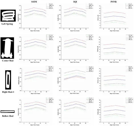
_{S S}E GT is the covariance

(11)

[image:11.595.64.535.96.539.2]

Figure-13. SSIM, IQI and PSNR for 4 parts with 4 segmentation algorithms for 80 frames.

Image Quality Index (IQI) is SSIM with

C

_SE



C

_SGT



0

. This parameter is useful in determining the pixel variations between the extracted and ground truth image. With no contrast terms in our case, indicates that the correlation between the pixels in the images. Finally, for defect identification PSNR in db plays a vital role, as it is difficult to predict the type of defects in real time. PSNR provides a value that tells the deviation in the detected defective from the perfectly working part. Since we used simulated defects for experimentation, the value of PSNR must be high for better Level set algorithm.

 









10

max max 10log

,

E

E GT

S PSNR

mse S S

 

 



 

 

(25)

SSIM values vary between 0 and 1. 0 represents the no similarity and 1 represents full similarity. IQI values tells the quality of the resulting image when compared to ground truth ranging from 0 to 1. PSNR gives the relationship between black and white pixels compared to ground truth. PSNR values indicates in dB changes from 3 to 13 dB for all bogie parts. For calculating small size of parts the PSNR value is small.

(12)

Figure-14. Rolling defects introduced in bogie parts using photoshop for testing the robustness of the proposed algorithms.

Plots in Figure-13 show a loss in value during first and last frames related to central frames. This is due to the reference frame used in the extraction of ground truth part. All the central frames were used for creation of ground truth parts. ISP_LS performs better compared to the other three models. SSIM and IQI touched 0.953 for ISP_LS and no other algorithm of the three reached that

score. PSNR for ISP_LS is around 12.93dB, which is again highest of the 4 segmenting algorithms.

(13)

Table-1. Mean SSIM, IQI and PSNR calculations for 4-trains at different timing of the day using the proposed level set models

Train Parts

SSIM IQI PSNR

CV_LS MDG_LS SP_LS ISP_LS CV_LS MDG_LS SP_LS ISP_LS CV_LS MDG_LS SP_LS ISP_LS

Train-1

Left Rod1 0.615 0.669 0.768 0.871 0.611 0.673 0.771 0.876 4.61 5.93 9.15 12.74 Left Rod2 0.638 0.675 0.781 0.882 0.641 0.681 0.774 0.872 4.83 6.01 9.27 12.59 Left Up 0.617 0.659 0.756 0.848 0.621 0.652 0.761 0.851 4.08 5.78 8.81 12.46 Left Spring 0.591 0.651 0.749 0.857 0.602 0.649 0.746 0.864 3.92 5.61 9.26 12.57 Center Rod 0.602 0.647 0.752 0.887 0.606 0.653 0.759 0.891 4.65 5.78 9.38 12.49

Right

Spring 0.599 0.661 0.759 0.862 0.593 0.663 0.763 0.861 4.06 5.27 9.29 12.65 Right Up 0.627 0.663 0.761 0.851 0.631 0.639 0.752 0.858 4.87 5.24 8.92 12.38 Right Rod2 0.631 0.679 0.774 0.879 0.639 0.671 0.781 0.877 4.97 5.58 9.09 12.29 Right Rod1 0.6232 0.6723 0.778 0.873 0.625 0.676 0.773 0.876 4.72 5.99 9.21 12.56 Bellow Rod 0.625 0.669 0.761 0.871 0.631 0.676 0.778 0.881 4.69 6.04 9.51 12.93

Train-2 (Night)

Right

Train-3 (Morning)

Right

Train-4 (Evening)

Right

(14)

The table gives mean values per part for the whole train. Every train consists of 15 coaches with 30 bogies. All the values are averaged per train. Comparing the 4 segmentation algorithms from the scores show a clear winner in the form of ISP_LS (Invariance Shape Prior Level Sets). The reason for its success depends on the control the model has over the sub-space of the shape model.

Our final study tries to estimate the robustness of the proposed methods on defective part segmentation. During the data capture phase, we could not locate any

defective components on the trains. Hence to test our segmentation models, we induced 9 defects in various critical parts using Photoshop software on the video frames. The 9 defects are shown in Figure-14.

The resulting segmented frames from the 4 algorithms are tested against the corresponding ground truth images. Defect identification with the proposed level set models is evaluated using SSIM, IQI and PSNR per video frame. Figure-15 gives evaluation plots for the 4 level set models with respect to SSIM, IQI and PSNR per defective part frame for 4 different defects.

Figure-15. SSIM, IQI and PSNR for four defective parts.

Plots in Figure-15 show ISP_LS performs better for defective part segmentation which is same as healthy parts. The figure shows two simple defects on rods and two complex defects on springs. All the experiments using ISP_LS use non-defective part to segment the defective part. This is done by reducing the value of , which

controls the shape energy of the level set. For defective parts having simple structure such as rods, the value of

0.23

(15)

contour on the image plane to extract the defect. The average SSIM in the case of complex structures like springs is averaged to 0.9001. This is due to self – occlusion during the train movement in the video frame.

[image:15.595.99.498.152.410.2]

SSIM, IQI and PSNR show CV-SI superiority in producing quality segmentations of defective parts during bogie transit.

Figure-16. Mean iterative rates for 9 induced defective bogie parts.

(a) SSIM (b) IQI (c) PSNR

Figure-17. Average (a) SSIM, (b) IQI and (c) PSNR for 4 segmenting algorithms used on 9 induced defective bogie parts.

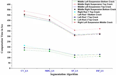
The average CPU time in seconds for 80 frames of 9 defective parts are shown in figure 16. CPU times vary based on the structural complexity of the part. From figure 16, the average CPU time for ISP_LS model is 150sec for simple rods in the bogie and 350sec for complex structures such as springs. Finally, figure 17 shows averaged SSIM, IQI and PSNR for the entire train captured at different times of the day with induced defective bogie parts. The 3D plots indicate that the complex parts like springs and the defects in them are segmented effectively using ISP_LS from a moving bogie compared to CV_LS, MDG_LS and SP_LS. Shape

invariance level sets are helpful in extracting defective parts irrespective of the type of defect or the location of defect in the bogie part.

[image:15.595.74.525.436.605.2]

(16)

pixels and impossible manual selection of foreground and background pixels in graph cuts due to closely packed pixels in a bogie part.

5. CONCLUSIONS

In this work, we try to find a workable 2D model to extract train bogie parts for computer vision based inspection of rolling stock. The methods used are Chan Vese level sets (CV_LS), Morphological Differential Gradient (MDG_LS), Shape Prior (SP_LS) and Invariance Shape Priors (ISP_LS) based level sets for rolling stock segmentation. The first two methods are global segmentation modules and the second two are local segmentation techniques. SSIM, IQI and PSNR are the parameters used to test the effectiveness of the models in extracting perfect bogie parts and defective bogie parts. Our findings show that, global segmentation on bogie parts using CV_LS and MDG_LS are slow and a manual identification is required to extract and identify each part. However, SP_LS and ISP_LS are faster and fully automated in extracting the bogie parts. ISP_LS is better than SP_LS in removing a constraint on the position, scale and alignment of the bogie part in the video. ISP_LS is robust in detecting defective parts compared to other three models. The local segmentation has a problem of part by part extraction of the train bogie there by reducing the speed of the algorithm for real time maintenance jobs.

REFERENCES

[1] Kishore P. and C.R. Prasad. 2017. Computer vision based train rolling stock examination. Optik-International Journal for Light and Electron Optics. 132: 427-444.

[2] Kishore P. and C.R. Prasad. 2015. Shape prior active contours for computerized vision based train rolling stock parts segmentation. International Review on Computers and Software (I. RE. CO. S.). 10: 1233-1243.

[3] Zhu S.C. and A. Yuille. 1996. Region competition: Unifying snakes, region growing, and Bayes/MDL for multiband image segmentation. IEEE transactions on pattern analysis and machine intelligence. 18(9): 884-900.

[4] Kishore P. V. V., D. Anil Kumar E. N. D., Goutham and M. Manikanta. 2016. Continuous sign language recognition from tracking and shape features using fuzzy inference engine. In Wireless Communications, Signal Processing and Networking (WiSPNET), International Conference on, pp. 2165-2170. IEEE.

[5] Kishore P. V. V., M. V. D. Prasad, D. Anil Kumar, and A. S. C. S. Sastry. 2016. Optical flow hand tracking and active contour hand shape features for

continuous sign language recognition with artificial neural networks. In Advanced Computing (IACC), 2016 IEEE 6th International Conference on, pp. 346-351. IEEE.

[6] Rao G. Ananth and P. V. V. Kishore. 2016. Sign language recognition system simulated for video captured with smart phone front camera. International Journal of Electrical and Computer Engineering. 6(5): 2176.

[7] Li Y., et al. 2017. Active contour model-based segmentation algorithm for medical robots recognition. Multimedia Tools and Applications. pp. 1-16.

[8] Kishore, P. V. V., M. V. D. Prasad, Ch Raghava Prasad, and R. Rahul. 2015. 4-Camera model for sign language recognition using elliptical fourier descriptors and ANN. In Signal Processing and Communication Engineering Systems (SPACES), 2015 International Conference on, pp. 34-38. IEEE.

[9] Kishore P. V. V., A. S. C. S. Sastry and A. Kartheek. 2014. Visual-verbal machine interpreter for sign language recognition under versatile video backgrounds. In Networks & Soft Computing (ICNSC), 2014 First International Conference on, pp. 135-140. IEEE.

[10]Kishore P. V. V., S. R. C. Kishore and M. V. D. Prasad. 2013. Conglomeration of hand shapes and texture information for recognizing gestures of Indian sign language using feed forward neural networks. International Journal of engineering and Technology (IJET) 5, no. 5 (2013): 3742-3756.

[11]Kishore P. V. V., D. Anil Kumar AS Chandra Sekhara Sastry and E. Kiran Kumar. 2018."Motionlets Matching with Adaptive Kernels for 3D Indian Sign Language Recognition. IEEE Sensors Journal.

[12]Kishore P. V. V. and Ch Raghava Prasad. 2015. Train rolling stock segmentation with morphological differential gradient active contours. In Advances in Computing. Communications and Informatics (ICACCI), 2015 International Conference on. pp. 1174-1178. IEEE.

(17)

Displacement Maps. IEEE Signal Processing Letters. 25(5): 645-649.

[14]Kosmopoulos D. and T. Varvarigou. 2001. Automated inspection of gaps on the automobile production line through stereo vision and specular reflection. Computers in Industry. 46(1): 49-63.

[15]Milanés V., et al. 2012. Intelligent automatic overtaking system using vision for vehicle detection. Expert Systems with Applications. 39(3): 3362-3373.

[16]Fathi H., F. Dai and M. Lourakis. 2015. Automated as-built 3D reconstruction of civil infrastructure using computer vision: Achievements, opportunities, and challenges. Advanced Engineering Informatics. 29(2): 149-161.

[17]Zhang H. and D. Li. 2014. Applications of computer vision techniques to cotton foreign matter inspection: A review. Computers and Electronics in Agriculture. 109: 59-70.

[18]Yang Y., et al. 2016. A robust vision inspection system for detecting surface defects of film capacitors. Signal Processing. 124: 54-62.

[19]Narayanaswami, S., Urban transportation: innovations in infrastructure planning and development. International Journal of Logistics Management, The. 28(1).

[20]Sabato A. and C. Niezrecki. 2017. Feasibility of digital image correlation for railroad tie inspection and ballast support assessment. Measurement, 2017. 103: p. 93-105.

[21]Hart J., et al. 2008. Machine vision using multi-spectral imaging for undercarriage inspection of railroad equipment. in Proceedings of the 8th World Congress on Railway Research, Seoul, Korea.

[22]Kim H. and W.-Y. Kim. 2011. Automated inspection system for rolling stock brake shoes. IEEE Transactions on Instrumentation and Measurement. 60(8): 2835-2847.

[23]Sanchez-Revuelta A.L. and C.-J.G. Gomez. 1998. Installation and process for measuring rolling parameters by means of artificial vision on wheels of railway vehicles. Google Patents.

[24]Kazanskiy N. and S. Popov. 2015. Integrated design technology for computer vision systems in railway

transportation. Pattern Recognition and Image Analysis. 25(2): 215-219.

[25]Freid B., et al. 2007. Multispectral machine vision for improved undercarriage inspection of railroad rolling stock. in Proceedings of the Ninth International Heavy Haul Conference Specialist Technical Session–High Tech in Heavy Haul, Kiruna, Sweden.

[26]Jarzebowicz L. and S. Judek. 2014. 3D machine vision system for inspection of contact strips in railway vehicle current collectors. in Applied Electronics (AE), 2014 International Conference on. IEEE.

[27]Zhang Y., et al. 2017. The application of WTP in 3-D reconstruction of train wheel surface and tread defect. Optik-International Journal for Light and Electron Optics. 131: 749-753.

[28]Kishore P., A. Sastry and Z.U. Rahman. 2016. Double Technique for Improving Ultrasound Medical Images. Journal of Medical Imaging and Health Informatics. 6(3): 667-675.

[29]Wang Z., et al. 2004. Image quality assessment: from error visibility to structural similarity. IEEE transactions on image processing. 13(4): 600-612.

[30]Terzopoulos D., et al. 1987. Elastically deformable models. in ACM Siggraph Computer Graphics. ACM.

[31]Kass M., A. Witkin and D. Terzopoulos. 1988. Snakes: Active contour models. International journal of computer vision. 1(4): 321-331.

[32]Chan T.F. and L.A. Vese. 2001. Active contours without edges. IEEE Transactions on image processing. 10(2): 266-277.

[33]Mumford D. and J. Shah. 1989. Optimal approximations by piecewise smooth functions and associated variational problems. Communications on pure and applied mathematics. 42(5): 577-685.

[34]Jiang N.Z.X. and X. Lan. 2006. Advances in Machine Vision, Image Processing, and Pattern Analysis.

[35]Huang X., H. Bai and S. Li. 2014. Automatic aerial image segmentation using a modified chan-vese algorithm. in Industrial Electronics and Applications (ICIEA), 2014 IEEE 9th Conference on. IEEE.

(18)

active contours. in Advances in Computing, Communications and Informatics (ICACCI), 2015 International Conference on. IEEE.

[37]Cremers D., S.J. Osher and S. Soatto. 2006. Kernel density estimation and intrinsic alignment for shape priors in level set segmentation. International journal of computer vision. 69(3): 335-351.

[38]Cremers D., N. Sochen and C. Schnörr. 2006. A multiphase dynamic labeling model for variational recognition-driven image segmentation. International Journal of Computer Vision. 66(1): 67-81.

[39]Sussman M., P. Smereka and S. Osher. 1994. A level set approach for computing solutions to incompressible two-phase flow. Journal of Computational physics. 114(1): 146-159.

[40]Laadhari A., P. Saramito and C. Misbah. 2016. An adaptive finite element method for the modeling of the equilibrium of red blood cells. International Journal for Numerical Methods in Fluids. 80(7): 397-428.

[41]Charpiat G., et al. 2006. Approximations of shape metrics and application to shape warping and empirical shape statistics, in Statistics and analysis of shapes. Springer. pp. 363-395.

[42]Madhav B., et al. 2015. Image enhancement using virtual contrast image fusion on Fe3O4 and ZnO nanodispersed decyloxy benzoic acid. Liquid Crystals. 42(9): 1329-1336.

[43]Farag A., et al. 2017. A Bottom-up Approach for Pancreas Segmentation using Cascaded Super pixels and (Deep) Image Patch Labeling. IEEE Transactions on Image Processing. 26(1): 386-399.