Space and Time Analysis on the Lattice of Cuboid for
Data Warehouse
Anjana Gosain
University school of Information Technology, GGSIPU, New Delhi-110006, India
Suman Mann
Maharaja Surajmal Institute of Technology, GGSIPU, New delhi-110006, India
ABSTRACT
Multidimensional analysis requires the computation of many aggregate functions over a large volume of collected data. To provide the various viewpoints for the analysts, these data are organized as a multi-dimensional data model called data cubes. Each cell in a data cube represents a unique set of values for the different dimensions and contains the metrics of interest. The different abstraction and concretization associated with a dimension may be represented as lattice. The focus is to move up and drill down within the lattice using an algorithm with optimal space and computation. In the lattice of cuboids, there exist multiple paths for summarization from a lower to an upper level of cuboid. The alternate paths involve different amounts of storage space and different volume of computations. Thus objective of this paper is to design an algorithm for formal analysis leading towards detection of an optimal path for any two given valid pair of cuboids at different levels. Algorithm is proposed based on branch and bound method for selection of optimal path. Experimental results in the last show that the solution obtained by the algorithm gives the optimal solution in terms of space and time computation.
Keywords:
Multidimensional Database, Data Cube, Cuboid, Lattice, Branch and Bound.1.
Introduction
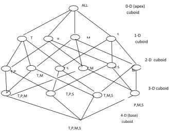
[image:1.595.122.475.491.746.2]A data warehouse (DW) is a repository of integrated information available for querying and analysis. The information in the data warehouse is stored in the form of multidimensional model[23]. The multidimensional model view data in the form of data cube. Data cube computes the aggregates along all possible combinations of dimensions [5]. It is defined by dimensions and facts. Dimensions are the entities with respect to which an organization wants to keep records [4]. Facts are the numerical measures/ quantities by which we want to analyze relationship between dimensions [20]. In general term we consider data cube as 3-D geometric structures, but in data warehousing it is n-dimensional [23]. The data cube is a metaphor for multidimensional data storage. Each cell of data cube shows a specific view in which users are interested. Given a set of dimensions, we can generate a cuboid for each of the possible subsets of the given dimensions which result in a lattice of cuboid. Figure 1 shows a lattice of cuboid for the dimensions time, product, market and supplier. For the n number of dimensions we may find 2n cuboid and main challenge is to understand how the cuboids are related to each
Figure 1. Lattice of Cuboid
P,M,S ALL
P
S M
T
T,P,M,S T,P,M
T.P
T,M,S T,P,S
T,M
T,S P,S M
,S P,M
0-D (apex) cuboid
1-D cuboid
2-D cuboid
3-D cuboid
other[3]. As shown in figure1 different paths are available for a particular cuboid. These paths consider different amount of storage space and time computation. Various researchers proposed number of algorithms for the selection and computation of data cubes [3][4][12][13][21][22]. In this paper an algorithm is proposed for computing the cuboid that minimizes the storage space and computation. Algorithm is proposed based on branch and bound method for selection of optimal path. The proposed algorithm gives the optimal solution in terms of space and time computation.
Rest of the paper is organized as follows: Section 2, presents the related works. Section 3, discusses definitions and properties related to lattice. Section 4, defines lemmas related to cube lattice. Section 5, presents the algorithm for cube computation. Section 6, explains the implementation of the proposed algorithm. Section 7, shows the result. Last section presents the conclusion.
2.Related Work
There has been some concurrent work on the problem of computing and selection of data cube [23][3][6][20][4][25]. V. Harinarayan et al. [23] proposed a greedy algorithm that work on lattice and pick the right views to materialize, subject to various constraints for the selection of data cube. A. Shukla et al. [2] proposed a modified greedy algorithm namely PBS (pick by size) that selects data cube according to the cube size. This algorithm was more efficient as compared to Harinarayan’s greedy algorithm. A polynomial time greedy heuristic framework that uses AND view (each view has a unique evaluation), OR view (any view can be computed from any of its related views), and AND-OR view graph is proposed by H. Gupta [7]. A. Shukla et al. [1] considered the view selection problem for multi-cube data models and proposed three different algorithms, SimpleLocal, SimpleGlobal, and ComplexGlobal which pick aggregates for precomputation from multi cube schemas. C. Zhang et al. [4] proposed a heuristic algorithm for determining a set of materialized views based on the idea of reusing temporary results from the execution of global queries with the help of Multiple View Processing Plan (MVPP). However, this algorithm did not consider the system storage constraints. Himanshu Gupta et al. [8] designed an approximation greedy algorithm for the special case of OR view graphs. For the general case of AND-OR view graphs, they also designed A*heuristic that deliver an optimal solution.
J. Yang et al. [4] used, Genetic Algorithm, to choose materialized views and demonstrate that it is practical and effective as compared to heuristic approaches. Again to select the set of materialized cubes W. Yang [15] proposed a greedy-repaired genetic algorithm and found that solution can greatly reduce the amount of query cost as well as the cube maintenance cost. A constraint programming based approach has been presented by I. Mami et al. [9] to address the view selection problem. More specifically, the view selection problem has been modeled as a constraint satisfaction problem. Its resolution has been supported automatically by constraint solver embedded in the constraint programming language. The authors proved experimentally that a constraint programming based approach provides better performances compared with a genetic algorithm (randomized) in term of the solution quality and cost saving. K. Aouiche et al. [14] proposed a framework for materialized view selection that exploits a data mining technique (clustering), in order to determine clusters of similar queries. They also proposed a view merging algorithm that builds a set of candidate views, as well as a greedy process for
selecting a set of views to materialize. Surveys of technique for selection of cube are given by the I. Mami [10].
For computing the cube, M.P. Deshpande [2][16] proposed a sorting based algorithm that overlap the computation of different group-by operations using the least possible memory for each computation of cube in the lattice of cuboid. Object oriented conceptual model based data cube is designed by A Lvanova and R. Boris [11]. For finding the optimal path in the lattice of cuboid, an algorithm proposed by S. Sen [21][22] is based on two operations roll-up and drill-down for finding the optimized path to traverse between two data cube of valid dimension in term of intermediate cuboid sizes. A galois connection is identified on the lattice structure with the well defined abstraction and concretization function based on the concept hierarchy. Recently researchers are focusing on designing efficient algorithms for the computation of the complete cube. In this paper we have proposed an algorithm for cube computation based on branch and bound technique.
3. Definition and Properties of Lattice
Theory
Some important definitions related to lattice are given below:
1. Lattice: A partial order set (POS) (A, ≤) is called a lattice if, x, y ε A, there exist sup(x, y) and inf (x, y) [27]. For supermum we use the symbol and for infimum we use the symbol .In the lattice theory, these operations are called binary operations.
2. POS: Partially ordered set is a set with a binary relation ≤ that, for any x, y, and z, satisfies the following conditions:
(1) x ≤ x (reflexivity);
(2) if x ≤ y and y ≤ x, then x = y (anti_symmetry);
(3) if x ≤ y and y ≤ z, then x ≤ z (transitivity).
If, for a POS (A, ≤), x, y ε A: x ≤ y or y ≤ x, then this set is called a linearly ordered set, or chain.
3. Supremum or Least Upper Bound: Let (A, R) be a POS. An element l ε A is called supremum of a and b in A if and only if
i. aRl and bRl i.e. l is the upper bound of a and b.
ii. If an element l’ ε A such that aRl’ and bRl’then lRl’
That is if l’ is another upper bound of a and b then l’ is also the upper bound of l. Thus l is the least upper bound of a and b.
4. Greatest Lower Bound(GLB) or Infimum
Let (A, R) be a POS. An element l ε A is called infimum of a and b in A if and only if
i. lRa and lRb i.e. l is the lower bound of a and b.
ii. If there exist one element l’ ε A such that l’ is also a lower bound of a and b then l’Rl that is if l’is also a lower bound of a, b then l’ is the lower bound of l also i.e. l is the greatest of all lower bounds of a and b.
That is if l’ is another upper bound of a and b then l’ is also the upper bound of l. Thus l is the least upper bound of a and b.
reverse of roll-up operation. Drill down is realized by stepping down a concept hierarchy or adding a new dimension.
3.1 Some Characteristics of Lattices
If A is any lattice, then for any a, b, c ε L the following properties hold:
i. a a = a Idempotent Law
a a = a
ii. a (b c) = (a b) c Associative Law a (b c) = (a b) c
iii.a b = b a Commutative Law a b = b a
iv. a (a b) = a Absorption Law a (a b) = a
4. Lemmas of Cube Lattice
Lemma1. In the cube lattice, the possible number of combinations of dimensions in each level r may be defined by the following permutation formula:
C (n, r) =n! /r! (n-r)!
Here in the cube lattice n= number of maximum dimensions
r= no of dimension taken at any level
In the cube lattice we start from zero level and total number of level will be equal to maximum number of dimension.
Now from this formula we may find number of nodes at any level in the cube lattice. Suppose we have four dimensions like product, time, market, and promotion. For these four dimensions we may find the following information
1. Number of levels is 4 because total number of dimension is four.
2. Number of nodes at level 0 = 1 as C (4, 1) = 4! / 0! (4-0) != 1
3. Number of nodes at level 1 = 4 as C (4, 1) = 4! / 1! (4-1) != 4
4. Number of nodes at level 2= 6 as C (4, 2) = 4! / 2! (4-2) != 6
5. Number of nodes at level 3=4 as C (4, 3) = 4! / 3! (4-3) != 4
6. Number of nodes at level 4=1 as C (4, 4) = 4! / 4! (4-4) != 1
Lemma2. Total number of possible nodes in the cube lattice will be equal to 2n where n is the maximum number of
dimensions. For the lattice of four dimensions total nodes are 16.
Lemma3. The number of dimensions for a cube in level i is the n-i for the base cuboid on n dimensions.
Lemma4. The number of cuboid produced by any particular cuboid for the next level will be equal to number of dimension in that particular cuboid. For example suppose we have the cuboid ABCD then number of cuboid produced for the next level is equal to 4 namely BCD, ACD, ABD and ABC.
5. Computation of Data Cube
For Computation of each cube, there exist multiple paths for summarization from a lower to an upper level cuboid. The alternate paths involve different amount of memory and
different volume of computations. Our challenge is to find a path which take minimum space and minimum number of computation. Thus computation of cube is to find an optimal path in terms of number of computation and storage space.
Here we have proposed an algorithm using branch and bound designing approach for computing the data cube. Before defining the algorithm, let us take a brief discussion about the branch and bound approach.
5.1 Branch and Bound Approach
In this approach we search for a set of solutions or we ask for an optimal solution satisfying some constraints. The desired solution is expressed as an n-tuple
(x1, x2, ---xn) where xi is taken from some finite set Si. For
any problem constraint are divided into two categories:
1. Explicit constraint
2. Implicit constraint
1. Explicit constraint: These are the rules that restrict each xi to
take on values only from a given set. All tuples that satisfy the explicit constraints define a possible solution space for a particular problem[5].
2. Implicit Constraint: These are the rules that determine which of the tuple in the solution spaces satisfy the criterion functions[5]. Thus implicit constraints describe the way in which the xi must relate to each other.
Branch and bound algorithm determine problem solutions by systematically searching the solution space for the given problem. This search is facilitated by using a tree organization for the solution space.
Once tree is conceived, the problem is solved by systematically generating the problem states, determining which of these are solution states and finally find out which solution states are answer states. Every problem state starts with the root node and then generates other nodes. A node which has been generated and all of whose children have not yet been generated is called the E-node i.e. note being expanded. A dead node is a generated node which is not to be expanded further or all of whose children have been generated. Now bounding functions are used to kill live nodes without generating all their children. In the branch and bound technique E-node remains the E-node until it is dead.
5.2 Algorithm for Cube Computation
Before defining the algorithm, first we make the state space diagram of the problem. Our problem is finding the aggregation over the dimensions according to the user queries. Now suppose we have five dimensions, Product, Time, Market, Promotion and Supplier. State space diagram for these five dimensions is given in figure1.The constraint for the problem is:
Explicit Constraint: Each dimension xi to take only from a
given set of dimensions (x1,x2,- xn).
Implicit Constraint: An implicit constraint in our problem is that aggregation of dimensions according to the user queries must be present in the subset of cuboid while selecting the cuboid.
For selecting the path following algorithm is used, which gives smallest number of computation among all possible paths.
Algorithm
1. Initialize the parameters; 2. Define a recursive function () initialise subsets, index, i, j, k to 0 temp[]<-{1,1,1,1,1},number of dimensions
loop until i<totalno initialise k and flag to 0 do subsets++
loop until j<n if(i+index=j) then{} else
arr[i][k]<-a[j][0] if(arr[i][k]<-f[0] or arr[i][k]<-f[1]) do
flag++ k++; end loop if(flag=1) do
if(temp[i]<min) do min<-temp[i] smin<-value at that position
else temp[i]<-1 i<-i-1 tno<-tno-1 index<-index+1 nsub<-nsub-1
endif
3. Repeat the above step to n-l times and get desired path
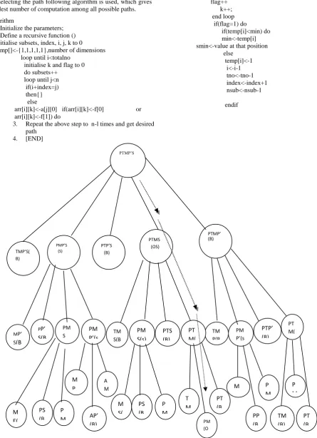
[image:4.595.72.518.75.690.2]4. [END]
Figure 2. State Space Diagram for Proposed Algorithm
PTMP’S
TMP’S( B)
PTMS (OS) PTP’S
(B) PMP’S
(S)
PTMP’ (B)
TM S(B
))
PM S(s)
PTS (B)
TM P(B
)
M S( B)
PS (B )
PM S (s)
9
(B)
MP’ S(B )
PP’ S(B )
PM P’(s )
PM P’(s )
PTP’ (B)
PT M( s)
PT M( os)
P M (S) P
M (S) PS (B ) M E( B)
AP’ (B)
A M
(B ) M
P (B)
M P’( B)
PM (O
S)
(O S)
PT (B ) T
M (B )
PP (B ) ’
P M (S)
TM (B)
P M (S)
6. Implementation
For implementing the algorithm, we have considered five dimensions i.e. Product (P), Time (T), Market (M), Promotion (P’) and Supplier (S) whose state space diagram is given in figure 2. In the state space diagram the solution nodes are represented by S and other nodes are represented by symbol B i.e bound. Now let us find the optimal path from (P, T, M, P’, S) to (P, M) i.e aggregation over product and market. (P, T, M, P’, S) is the base cube at lowest level. Let us suppose the attribute value of various dimensions, P has 25 values, T has 20 values, M has 35values, P’ has 40 values and S has 10 values. Our algorithm starts with materialization of base cuboid and then algorithm materialize the following cuboids:
1. T, M, P’, S
2. P,M, P’, S
3. P, T, P’, S
4. P,T,M,S
5. P,T,M,P’
Now in these options, algorithm will check the feasible solution and cuboid with minimum number of computation. Feasible solution is the cuboid that contain the dimension P,M. Number of computation is the multiplication of attribute value of considered cuboid. The cuboid which have the minimum number of computation in the above cuboid is P,T, M,S. Next this cube is materialized for getting the optimal solution and cuboid, from which the solution like T,M,P’,S is not possible will be bounded. Bound node is represented by inserting B in the materialized cuboid. Other nodes are the solution nodes, which are represented by putting S in the materialized cuboid.From P,T,M,S we get the following :
1. T, M, S
2. P, M, S
3. P, T, S
4. P, T, M
Here again it will check the feasible solution and in feasible solution will select the path with minimum number of computation which here is P, T, M. Now P, M, S will be selected and following option we get:
1. M,S
2. P, S
3. P, M
Now feasible solution is P,M and this is the required optimal path.This is represented by OS(optimal solution) in the state space diagram Thus selected path is:
(P, T, M, P’, S) P, T, M, S P, M, S P,M
Before applying the algorithm the possible solutions are the following:
1.P, T, M, P’,S P, M, P’,S P, M,S P, M 359625
2.P, T, M, P’,S P, M, P’,S P, M,P’ P, M 385875
3.P, T, M, P’,S P, T, M, S P, M,S P, M 184625(os)
4.P, T, M, P’,S P, T, M’,S P,T, M P, M 193375
5.P, T, M, P’,S P, T, M, P’ P, M,P’ P, M 735875
6.P, T, M, P’,S P, T, M, P’ P, T, M P, M 718375
In these options we see that 3rd alternative is optimal as compared to others in term of storage space and computation time. This same we get from our algorithm. The optimal solution is represented by the arrow line in state space diagram of figure 2.
7. Experimental Result
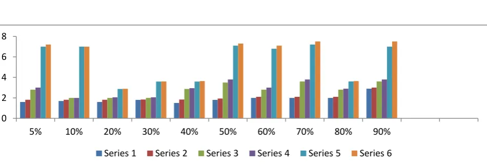
To validate the effectiveness of the proposed cube selection algorithm, we compared it with alternative path of cube selection. For this we find the aggregation of two dimensions over five dimensional cube. Two dimensional cubes are PT, PM, PP’, PS, TM, TP’, TS, MP’, MS, P’S. For these two dimensional cubes, we considered 10 different values set as 5%, 10%, 20%, 30%, 40%, 50%, 60%, 70%, 80%, 90% as a space utilization in memory. We have aggregated all two dimensions according to our proposed algorithm. For the same solution, we have aggregated according to their independent path. Then graph is made of the independent solutions and from the solution of our algorithm. This is depicted in figure3.
In figure 3 horizontal line shows the space limit and vertical line indicates the number of computation in lakhs. Blue line i.e. series 1 is the result of our algorithm. In this diagram, we may see the improvement over space as well as total response time in terms of number of computation. In the graph first blue line is the result of our algorithm, which is minimum for all the two dimensional aggregations i.e. PT, PM, PP’, PS, TM, TP’, TS, MP’, MS, P’S.
Figure3 Result Analysis of the Algorithm 0
2 4 6 8
5% 10% 20% 30% 40% 50% 60% 70% 80% 90%
[image:5.595.62.537.572.734.2]8. Conclusion
In this paper, we have analyzed the roll-up and drill-down operations on the multidimensional data cube. The proposed algorithm is based on the roll-up and drill-down operations for finding the optimized path to traverse between two data cube of valid dimensions in term of intermediate cuboid sizes.
References
[1] A. Shukla, Deshpande PM, Naughton JF, “materialized view selection for multicube data models” 7th
international conference on extended database technology, Germany, March 2000, Springer, pp 269-284.
[2] A. Shukla, PM Deshpande, JF Naughton, “materialized view selection for multidimensional datasets”, Proceeding of 24th
international conference on very large databases, NEW York, August 1998,pp 488-499.
[3] Antoaneta Ivanova, Boris Rachev, “Multidimensional models – Constructing data cube”, International Conference on Computer Systems and Technologies- CompSysTech’2004.
[4] C. Zhang and J. Yang, “Genetic algorithm for materialized view selection in data warehouse environments,” Proceedings of the International Conference on data Warehousing and Knowledge Discovery, LNCS, vol.1676,pp. 116-125, 1999
[5] Ellis Hororwitz, Sartaj Sahni, Sanguthevar Rajasekaran, "fundamentals of computer algorithms" Galgotia publication, 1999.
[6] G. Sanjay, C. Alok, “Parallel Data cube Construction for high performance On_line analytical processing”, IEEE .Inter. Confer.1997, pp10-14
[7] H. Gupta, “selection of views to materialize in a data Warehouse”, ICDT, January 1997, Delphi Greece.
[8] H. Gupta, I.S. Mumick, Selection of views to materialize under maintenance cost constraint. In Proc.7th International Conference on Database Theory (ICDT'99) Jerusalem, Israel, pp. 453–470, 1999
[9] I. Mami, R. Coletta, and Z. Bellahsene, “Modeling view selection as a constraint satisfaction problem”, In DEXA, pp 396-410,2011
[10]I. Mami and Z. Bellahsene,”A survey of view selection method” SIGMOD Record, March 2012 (Vol. 41, No. 1), pp 20-30
[11]I. Antoaneta, R Boris, “Multidimensional models-constructing data cube” Int. conference on computer systems and technologies-CompSysTech’2004, V-5pp1-7
[12]J.Hen, J.Pei,G.D and K. Wang, ‘Efffficient computation of iceberg cubes with complex measures,” in proc. 2001 ACM-SIGMOD Int. conference Management of data (SIGMOD’01),May2001,PP1-12.
[13]J.Yang, K. Karlapalem, and Q. Li. “A framework for designing materialized views in data warehousing environment”, proceedings of 17th IEEE International conference on Distributed Computing Systems, Maryland, U.S.A., May 1997
[14]K. Aouiche, P. Jouve, and J. Darmont. Clustering-based materialized view selection in data warehouses.In ADBIS’06, volume 4152 of LNCS, pages 81–95, 2006.
[15]L.Y.Wen, K.I. Chung, “A genetic algorithm for OLAP data cubes” Knowledge and information systems, January 2004,volume 6,Issue1,pp 83-102.
[16]M.P. Deshpande ,S.Agarwal, J.F. Naughton, R. Ramakrishnan “Computation of Multidimensional Aggregates” University of Wisconsin Madison, Technical Report,1997
[17]M.P. Deshpande, S.Agarwal, R.Agarwal, A. Gupta, J. F. Naughton,R. Ramakrishnan and S. Sarawagi; "On the computation of multidimensional aggregates"; Proc. of 1996 International Conference on Very Large Data Bases VLDB'96.
[18]S. Amit, D Prasad, N.F. Jeffrey, “Materialized view selection for multi-cube data models, In Proc. of 7th Int.conference on Extending database Technology: Advances in Database Technology, Springer 2000, pp 269-284.
[19]S.D.Kuznetsov, Y.A.Kudryavtsev,“ A mathematicl model of the OLAP cubes” Programming and computer software, vol35,no5,2009, pp 257-265.
[20]Stefanovic, N., Han, J., Koperski, K.: Object-Based Selective Materialization for efficient Implementation of Spatial data cubes. IEEE transaction on Knowledge and DataEngineering,2000,pp 938-958
[21]S. Soumya,C. Nabendu, C. Agostino, “Optimal space and time complexity analysis on the lattice of cuboids using galois connections for the data warehousing” In proc 2009,Inter.conf.on computer science and convergence information technology,pp1271- 1275.
[22]S. Soumya, C.Nabendu, “Efficient traversal in data warehouse based on concept hierarchy using Galois Connections, In proc. of second Int. Con on Emerging applicationsof information technology,2011,pp 335- 339
[23]V. Harinarayan, Rajaraman, A., Ullman,“ Implementing Data Cubes Efficiently”, In ACM SIGMOD International Conference on Management of Data, ACM Press, New York (1996) pp. 205-216.
[24]W.H.Inmon, “building the data warehouse” Wiley, Fourth Edition, 2005.
[25]X.Li, J.Han, and H. Gonzalez, “High dimensional OLAP: a Minimal cubing approach,”in Proc. 2004 Int.Conf.Very Large Databases (VLDB’04),Toronto Canada,Aug. 2004,pp. 528-539.
[26]Y.Chen, G. Dong,J.Han, B.W.Wah, and J.Wang, “Multidimensional regression analysis of time series data streams,” in proc.2002 International conference on very large data Bases(VLDB’02),Hong Cong, Chiana, Aug.2002,pp.323-334
[27]Y.A Kudryavtsev, S.D.Kuznetsov, “A Mathematical model of the OLAP cubes”,Programming and computer software,Vol35, No 5,2009, pp 257-265.
[28]Z. Shao., J.Han, and d.Xin, “MM-cubing: computing iceberg cubes by factorizing the lattice space,” In Proc.2004 Int. Conf. on Scientific and statistical Database Management (SSDBM’04), Santorini Island, Greece, June 2004,pp.213-22.