On Rayleigh-Ritz Method in Three-Parameter Eigenvalue
Problems
Surashmi Bhattacharyya Arun Kumar Baruah
Department of Mathematics Department of Mathematics Dibrugarh University,Assam, India Dibrugarh University, Assam, India
ABSTRACT
This paper deals with the computation of the eigenvalues of a three-parameter Sturm-Liouville problem in the form of ordinary differential equation using Rayleigh-Ritz Method, a method which is based on the principle of variational methods. This method has been effective in computing the eigenvalues of self-adjoint problems. The resulting equations obtained in applying Rayleigh-Ritz method on the problem are solved to find the rough estimates of the eigenvalues of the problem. Rough estimates are used as starting approximations in the corresponding shooting method to obtain their actual values.
Keywords
Eigenvalue, eigenfunction, multiparameter, variational method, Rayleigh-Ritz method.
1.
INTRODUCTION
The finite element method (FEM) is one of the most powerful technique for numerical treatment of differential equations. FEM is widely used in almost every field of engineering and applied sciences such as structural mechanics, fluid mechanics, electromagnetism etc. The FEM is based on the classical variational method combined with chosen analytical functions. This method is known as Rayleigh-Ritz method. Multiparameter eigenvalue problems (MPEVP’s) are generalization of one-parameter eigenvalue problems and arise when the method of separation of variables is applied to certain boundary value problems associated with partial differential equations.
One-parameter problems are much developed both theoretically and numerically. Extensive theoretical development of multiparameter eigenvalue problems found in [1], [2], [3], [4]. Also, several authors in their works [5], [6], [7], [8], [9], [10], [11] have dealt with numerical analysis of two-parameter eigenvalue problems. But theoretical and numerical investigation in three-parameter eigenvalue problems are still very few. In this paper, the three-parameter problem considered for numerical treatment is in the form of a linear ordinary differential equation given by
(1.1) subject to the four point boundary conditions
(1.2) where , and are given real valued continuous functions of the independent variable . The values of the parameters , and which are called eigenvalues for the problem, for which there is a non-trivial solution , called eigenfunction of (1.1)-(1.2). Accounts of existence of the eigenvalues for two-parameter problems can be found in [12]. The points at which vanishes in
, and are called zeros of the eigenfunction
. The function is said to be oscillatory in , and , if there exists at least one zero in the interval. Due to the boundary conditions imposed on the problem, always it is ensured of eigenfunctions which are at best oscillatory in this case [13].
In this paper a brief account of the method used is given. The starting values of the eigenvalues are obtained by solving the algebraic equations obtained on application of Rayleigh-Ritz method. Using these starting values in the corresponding shooting method of the problem, actual values are obtained. The shooting method requires good starting values because the convergence and its rapidity both depend on starting values. Shooting method of [10] is extended to treat the problem (1.1)-(1.2) numerically in the present case.
2.
VARIATIONAL METHOD
The problem in which it is often possible to replace the problem of integrating a differential equation by the equivalent problem of seeking a function that gives a minimum value of some integral are called variational problem. The method that allows to reduce the problem of integrating a differential equation to the equivalent variational problem are usually called variational methods.
The variational methods are approximate methods based on the criterion of the calculus of variations. The method is concerned with seeking the extremum (minima or maxima) of an integral expression involving a function of functions or functional. In the calculus of variations, one is interested in finding the necessary condition for a functional to achieve a stationary value. This necessary condition on the functional is generally in the form of differential equation with boundary conditions on the required function. The function for which the integral attains its minimum value is the solution of the given differential equation.
Consider the problem of finding a function such that the function[14],
(2.1)
subject to the boundary conditions,
, (2.2) takes a maximum or minimum value. The integrand is a
function of , and its derivative . is called functional. The problem here is finding an extremizing function for which the functional has an extremum.
Let is a given function possessing continuous partial derivatives with respect to each of its arguments. Also let
is continuous and has a continuous derivative in the interval .
39
is a function for which the integral (2.1) will be greater or less than for any other function with continuous derivative in and prescribed values (2.2).
Any function in the neighborhood of may be written as
(2.3) where is an arbitrary parameter and is an arbitrary function with continuous derivatives in and , (2.4) Now, on replacing in (2.1) by , the equation can be obtained as,
(2.5)
where denotes the new integral value. The functional
is a function of and attains a maximum and minimum value at . Hence, the first derivative of with respect to becomes zero at , such that
(2.6) Integrating by parts the second term on the right-hand side of
(2.6) and using (2.4), the equation can be obtained as
(2.7)
Lemma 2.1
If in the integral(2.8)
the function is continuous between and and if the integral vanishes for all function which are continuously differentiable and vanishes at and , then must be identically zero in the interval.
Using this lemma from (2.7), the result that if maximizes or minimizes the integral (2.1), it must satisfy the condition
(2.9)
The Eq. (2.9) is called the Euler equation.
3.
RAYLEIGH-RITZ METHOD
Variational methods can be classified as direct and indirect methods. The classical Rayleigh-Ritz method belongs to the direct variational method as it is the direct application of variational principle based on the minimization of a given functional. The method of Weighted Residuals fall under the indirect variational methods, namely, collocation, sub-domain, Galerkin and least square methods etc.
The method was first presented by Rayleigh in 1877 and extended by Ritz in 1909 as found in [15]. This method can be applied to only self-adjoint problems.
In this method, first a linearly independent set of functions called basis functions are selected and then constructed an approximate solution to the Eq. (2.1), satisfying some prescribed boundary conditions. The approximate solution is in the form
(3.1) where are arbitrary parameters and and are prescribed functions satisfying inhomogeneous and homogeneous boundary conditions respectively of the given boundary value problem. Since the essential boundary conditions on both ends are homogeneous, .
Substituting (3.1) in (2.1), the integral can be obtained as
(3.2) The minimum of this function is obtained when its partial derivatives with respect to coefficients are zero :
, (3.3)
The system (3.3) obtained above is a set of simultaneous equations. The system of linear or non-linear algebraic equations obtained are solved to get the parameters , which are finally substituted into the approximate solution of the Eq. (3.1).
If possess continuous second order derivatives, then by integrating by parts the first term in the integrand of (3.3) gives,
, (3.4)
For the differential equation
(3.5)
with the boundary conditions (2.2), it can be verified that with
(3.6) the Euler equation (2.9) is identical with the given differential equation (3.5).
4.
SELF-ADJOINT OPERATOR
An operator is said to be self-adjoint if . Sturm-Liouville operator is a well known self-adjoint operator. Using differential operator the general homogeneous linear ODE of order can be written as,
(4.1)
where denote the differential operator. Further, if the operator is self-adjoint then,
(4.2)
The problem considered in (1.1) can be written as,
, (4.3)
(4.4) Since, , hence the problem is a self-adjoint one. The importance of the self-adjointness lies in the result that if a differential operator is self-adjoint then all eigenvalues of the operator are real and eigenfunctions are orthogonal.
5.
ILLUSTRATIVE EXAMPLE
The numerical example of the problem (1.1)-(1.2) considered here is a boundary value problem in the form of generalised Mathieu’s equation found in [16] :
(5.1) subject to the boundary conditions
(5.2)
The integrand corresponding to the given differential equation (5.1) is
(5.3) Since with defined by (5.3) the Euler equation (2.9) is identical with the given differential equation (5.1). Using (2.1) and (5.3), the three variational problems can be obtained as:
(5.4)
(5.5)
(5.6)
where satisfies the boundary conditions (5.2).
The approximate solution of (5.1) satisfying the boundary condition (5.2) is chosen as,
(5.7)
Following values are now easy derivations :
(5.8)
(5.9)
(5.10) Therefore, the functional in in and
in become
(5.11)
(5.12)
(5.13)
For minimization of , and , differentiaing (5.11), (5.12) and (5.13) with respect to , and following equations are obtained.
(5.14)
41
(5.15)
(5.16)
(5.17)
(5.18)
(5.19)
(5.20)
(5.21)
(5.22)
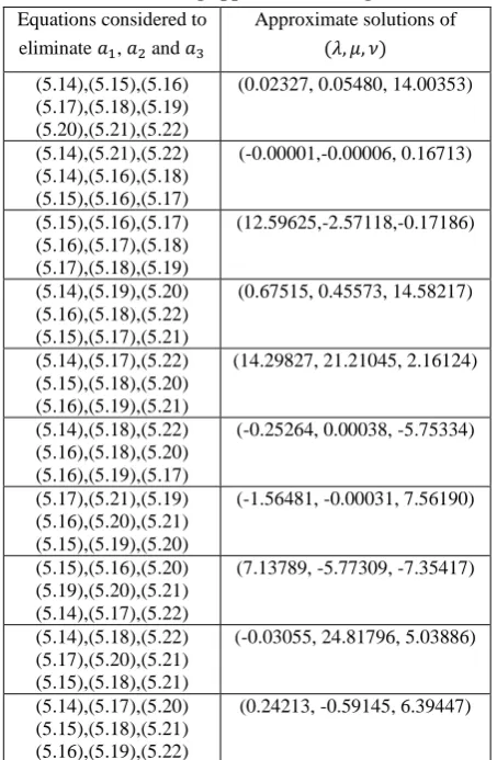
[image:4.595.314.541.82.429.2]Eliminating , and from the above equations taking three at a time different algebraic equations can be obtained. Solving those algebraic equations [17, 18], different sets of starting values of the eigenvalues of the problem (5.1)-(5.2) are obtained as shown in Table - 1 below :
Table 1. Starting appox. for shooting method
Equations considered to eliminate , and
Approximate solutions of
(5.14),(5.15),(5.16) (5.17),(5.18),(5.19) (5.20),(5.21),(5.22)
(0.02327, 0.05480, 14.00353)
(5.14),(5.21),(5.22) (5.14),(5.16),(5.18) (5.15),(5.16),(5.17)
(-0.00001,-0.00006, 0.16713)
(5.15),(5.16),(5.17) (5.16),(5.17),(5.18) (5.17),(5.18),(5.19)
(12.59625,-2.57118,-0.17186)
(5.14),(5.19),(5.20) (5.16),(5.18),(5.22) (5.15),(5.17),(5.21)
(0.67515, 0.45573, 14.58217)
(5.14),(5.17),(5.22) (5.15),(5.18),(5.20) (5.16),(5.19),(5.21)
(14.29827, 21.21045, 2.16124)
(5.14),(5.18),(5.22) (5.16),(5.18),(5.20) (5.16),(5.19),(5.17)
(-0.25264, 0.00038, -5.75334)
(5.17),(5.21),(5.19) (5.16),(5.20),(5.21) (5.15),(5.19),(5.20)
(-1.56481, -0.00031, 7.56190)
(5.15),(5.16),(5.20) (5.19),(5.20),(5.21) (5.14),(5.17),(5.22)
(7.13789, -5.77309, -7.35417)
(5.14),(5.18),(5.22) (5.17),(5.20),(5.21) (5.15),(5.18),(5.21)
(-0.03055, 24.81796, 5.03886)
(5.14),(5.17),(5.20) (5.15),(5.18),(5.21) (5.16),(5.19),(5.22)
(0.24213, -0.59145, 6.39447)
The starting values of the eigenvalues obtained from the
Table -1 are used in the corresponding shooting method of
the problem to obtain the actual values of the eigenvalues. The distinct actual values of the eigenvalues of the problem (5.1)-(5.2) are found as (9.85032, 1.17066, 0.21466), (16.55933, 5.64528, -12.95556), (94.62722, 1.55593, -40.89388), (31.86222, 1.61774, 13.06382), (37.99081, -22.74049, 12.21601), (28.65122, 10.66956, 8.80906), the corresponding eigenfunctions of which has number of zeros in the intervals (0, 1), (1, 2) and (2, 3) as (0, 0, 0), (0, 2, 1), (2, 4, 3), (2, 0, 2), (0, 0, 3), (2, 1, 1) respectively.
6.
CONCLUSIONS
In this paper, eigenvalues of three-parameter problem in the form of ordinary differential equation are computed using Rayleigh-Ritz method, a method which is very effective in computing eigenvalues of self-adjoint problems. Here, it is observed that starting values of the eigenvalues are dependent on the choice of approximate solution . The problem (1.1)-(1.2) defined in the interval are considered separately in the intervals , and so that enough algebraic equations can be generated for finding unknowns together with , and .
7.
REFERENCES
[2] Atkinson, F. V. 1968. Multiparameter spectral theory, Bull. Am. Math. Soc., 75, (1-28).
[3] Sleeman, B. D. 1972. The two-parameter Sturm-Liouville problem for ordinary differential equations, II, Proc. of the American Math. Soc vol. 34(1), 165-170.
[4] Browne, P. J. 1972. A multiparameter eigenvalue problem, J. Math. Analysis and Appl., 38, 553-568.
[5] Baruah, A. K. 1987. Estimation of eigen elements in a two- parameter eigenvalue problem, Ph. D. Thesis, Dibrugarh University, Assam.
[6] Baruah, A. K. 2012. Ritz method in multiparameter eigenvalue problem, IFRSA’s International of Computing, Vol.2(1), 156-162.
[7] Konwar, J. 2002. Certain studies of two-parameter eigenvalue problem, Ph. D. thesis, Dibrugarh University, Assam.
[8] Changmai, J. 2009. Study of two-parameter eigenvalue problem in the light of finite element procedure, Ph. D thesis, Dibrugarh University, Assam.
[9] Plestanjak, B. 2006. Multiparameter eigenvalue problems, 2nd International Conference on Structural Matrices, Hongkong Baptist University.
[10] Fox, L., Hayes, L. And Mayers, D. F. 1972. The double eigenvalue problem : Topics in numerical analysis, Proc.
Roy Irish Acad. Con., Univ. College, Dublin, Academic Press, New York, London, 93-112.
[11] Chanane, B., and Boucherif, A. 2012. Two-parameter Sturm-Liouville problems, ar Xiv:1208.3695v1 [math.SP]. King Fahd University of Petroleum and Minerals, Dhahran 31261, Saudi Arabia.
[12] Gregus, M., Nueman, F. and Arscott, F.M. 1971. Three point boundary value problems in differential equation, J, London Math. Soc(2),3, 429-436. [13] Sleeman, B. D., 1972. Completeness and expansion
theorems for a two-parameter eigenvalue problem in ordinary differential equations using variational principles, J., London Math. Soc.(2),6, 705-712.
[14] Jain, M. K., 1983. Numerical solution of differential equations, Wiley Eastern Ltd.,New-Delhi, 522-528. [15] Sadiku, M. N. O. 2001. Numerical Techniques in
Electromagnetics, CRC Press, 235-274.
[16] Collatz, L. 1968. Multiparameter eigenvalue problem in Inner Product Spaces , J. Compu. and Syst. Scie., 2, 333-341.
[17] Rao, K. S. 2007. Numerical methods for scientists and engineers, Prentices-Hall of India(P) Ltd.