Alternating Group Explicit Iterative Methods for One Dimensional Advection Diffusion Equation

(1)

http://dx.doi.org/10.4236/ajcm.2015.53025

How to cite this paper: Chen, N. and Gu, H.M. (2015) Alternating Group Explicit Iterative Methods for One-Dimensional Advection-Diffusion Equation. American Journal of Computational Mathematics, 5, 274-282.

http://dx.doi.org/10.4236/ajcm.2015.53025

Alternating Group Explicit Iterative Methods

for One-Dimensional Advection-Diffusion

Equation

Ning Chen, Haiming Gu*

College of Mathematics and Physics, Qingdao University of Science and Technology, Qingdao, China Email: *_{[email protected]}

Received 30 June 2015; accepted 28 August 2015; published 31 August 2015

This work is licensed under the Creative Commons Attribution International License (CC BY). http://creativecommons.org/licenses/by/4.0/

Abstract

The finite difference method such as alternating group iterative methods is useful in numerical method for evolutionary equations and this is the standard approach taken in this paper. Alter-nating group explicit (AGE) iterative methods for one-dimensional convection diffusion equations problems are given. The stability and convergence are analyzed by the linear method. Numerical results of the model problem are taken. Known test problems have been studied to demonstrate the accuracy of the method. Numerical results show that the behavior of the method with empha-sis on treatment of boundary conditions is valuable.

Keywords

One-Dimensional Advection-Diffusion Equations, Alternating Group Explicit Iterative Methods, Stability, Convergence, Finite Difference Method

1. Introduction

In this paper, we consider the one-dimensional time-dependent advection-diffusion equations

( )

2

1

2

0

, 0 , 0

0, , 0

1, , 0

, 0 , 0

u u u

a b x L t T

t x x

u t g t t T

u t g t t T

u x u x x L

∂ ∂ ∂

+ = < < < <

 ∂ ∂ ∂

 ₌ _{< <}



 ₌ _{< <}



= < <



(1)

*

(2)

where u0

( ) ( ) ( )

x ,g t1 ,g2 t are known functions while the function u is unknown; a and b are positive

constants quantifying the diffusion and advection processes, respectively. Equation (1) describes advection-diffusion of quantities such as heat, energy, mass, etc. They find their application in water transfer in soils, heat transfer in draining film, spread of pollutants in rivers and dispersion of tracers in porous media. They are also widely used in studying the spread of solute in a liquid flowing through a tube, long-range transport of pollutants in the atmosphere, flow in porous media and many others (see [1] [2]). This method has been applied and ana-lyzed for the Timoshenko beam problem, the Reissner-Mindlin plate, the arch problem and the ax symmetric shell problem. As a major contribution for these mixed formulations, this method has overcome the difficulties concerning the usual stability conditions allowing combinations of simple finite element polynomials of almost any order including the attractive equal-order interpolations.

They are also important in many branches of engineering and applied science. These equations are characte-rized by a non-dissipative (hyperbolic) advective transport component and a dissipative (parabolic) diffusive component. All numerical profiles go well when diffusion is the dominant factor. On the contrary, when advec-tion is dominant transport process, most numerical results exhibit some combinaadvec-tion of spurious oscillaadvec-tions and excessive numerical diffusion. These behaviors can be easily explained using a general Fourier analysis. Little progress has been made to overcome such difficulties effectively. Using extremely fine mesh is one alternative but is not prudent to apply it as it is computationally costlier. So a great effort has been made on developing the efficient and stable numerical techniques.

The numerical methods that have been applied to advection-diffusion equation include finite difference me-thods, Galerkin meme-thods, spectral meme-thods, wavelet based finite elements and several others. The AGE method is an iterative method employing the fractional splitting strategy which is applied alternately at each interme-diate step on tridiagonal system of difference schemes. Its rate of convergence is governed by the acceleration parameter r. The AGE iterative method is applied to a variety of problems involving parabolic and hyperbolic partial differential equations (see [3]-[6]). In [7], Sahimi and Evans reformulated the AGE method to solve the Navier-Stokes equations in the stream function-vorticity form. In this paper we apply the AGE iterative method to the one-dimensional advection diffusion equation. We put forward a new iterative method by numerical dif-ferentiation and also extend the original method. The AGE method is shown to be extremely powerful and flexi-ble and affords its users many advantages. Computational results are obtained to demonstrate the applicability of the method on some problems with known solutions.

2. Finite Difference Discretization

Let us divide the domain K=

[ ]

1,N into N equal sized elements of length h=L N . The N+1 nodes have coordinates xi with i=1, 2,,N. The discrete solution consists of nodal values of the function ui,

which approximate the exact solution at the nodes xi. We denote τ=tn+1−tn be time interval, n i

U be ap-proximation solution, where xi = −

( )

i 1 ,h i=1, 2,,m+1; tn=nτ, n=0,1,,J=

[ ]

T τ . Let

2

r=τ h to be a ratio of mesh sizes. In this paper, we special discuss the AGE methods for m=8 ,J h=L m.

Introduce the following fourth order difference form as

(

)

1

1 1 1 1 1 1

2 2

1 1 1 1 2 2 2 2

2 2 2 2 2

2 4

2 2 2 2

1 4 1

2 3 3 4 4

,

n _n _n _n _n _n _n _n _n _n _n _n _n

i i i i i i i i i i i i

i

u u u u u u u u u u u u

u

x h h h h

O τ h

+ ₊ ₊ ₊ ₊ ₊ ₊

+ − + − + − + −

    

∂  ₌  _⋅ − + ₊ − + ₋ − + ₊ − +



_∂     



      

+ +

(2)

( )

1 1 2

2

n n n

i i

i

u u

u

O τ

τ τ

+ + ₋

∂

  ₌ ₊

_∂ 

  (3)

Applying the second class Saul’yev asymmetric difference schemes (see [8]), this leads to the following eight difference form based eight internal grid points as

(

)

(

)

(

)

(

)

(

)

(

)

(

)

(

)

1 1 1

1 2

2 1 1 2

1 15 8 2

2 16 2 1 45 8 2 ,

n n n

i i i

n n n n n

i i i i i

br U r b ah U r b ah U

r b ah U r b ah U br U r b ah U r b ah U

+ + +

+ +

− − + +

+ − − + −

(3)

(

)

(

)

(

)

(

)

(

)

(

)

(

)

(

)

(

)

1 1 1 1

1 1 2

2 1 1 2

8 2 1 31 8 2

2 8 2 1 29 8 2 ,

n n n n

i i i i

n n n n n

i i i i i

r b ah U br U r b ah U r b ah U

+ + + +

− + +

− − + +

− + + + − − + −

= − + + + + − + − − − (5)

(

)

(

)

(

)

(

)

(

)

(

)

(

)

(

)

(

)

1 1 1 1

1 1 2

2 1 1 2

8 2 1 29 8 2

2 8 2 1 29 8 2 ,

n n n n

i i i i

n n n n n

i i i i i

+ + + +

− + +

− − + +

− + + + − − + −

= − + + + + − + − − − (6)

(

)

(

)

(

)

(

)

(

)

(

)

(

)

(

)

1 1 1 1 1

2 1 1 2

2 1

8 2 1 45 16 2 2

8 2 1 15 ,

n n n n n

i i i i i

n n n

i i i

r b ah U r b ah U br U

+ + + + +

− − + +

− −

+ − + + + − − + −

= − + + + + − (7)

(

)

(

)

(

)

(

)

(

)

(

)

(

)

(

)

1 1 1 1 1

2 1 1 2

1 2

2 16 2 1 45 8 2

1 15 8 2 ,

n n n n n

i i i i i

n n n

i i i

+ + + + +

− − + +

+ +

+ − + + + − − + −

= − + − − − (8)

(

)

(

)

(

)

(

)

(

)

(

)

(

)

(

)

(

)

1 1 1 1 1

2 1 1 2

1 1 2

2 8 2 1 29 8 2

8 2 1 31 8 2 ,

n n n n n

i i i i i

n n n n

i i i i

+ + + + +

− − + +

− + +

+ − + + + − − + −

= + + − + − − − (9)

(

)

(

)

(

)

(

)

(

)

(

)

(

)

(

)

(

)

1 1 1 1

2 1 1

2 1 1 2

8 2 1 31 8 2

8 2 1 29 8 2 2 ,

n n n n

i i i i

n n n n n

i i i i i

r b ah U r b ah U br U r b ah U

+ + + +

− − +

− − + +

+ − + + + − −

= − + + + + − + − − − (10)

(

)

(

)

(

)

(

)

(

)

(

)

(

)

(

)

1 1 1

2 1

2 1 1 2

8 2 1 15

8 2 1 45 16 2 2 .

n n n

i i i

n n n n n

i i i i i

+ + +

− −

− − + +

+ − + + +

= − + + + + − + − − − (11)

3. AGE Iterative Methods

Now, we can construct AGE iterative forms based on (4)-(11). Let m=8J. For the time level n, if n can be odds, the grid points will be divided into J parts. Know that there are eight grid points in each part, and then, we will apply the form (4), (5), …, (11) to find the solution one by one. If n can be evens, the grid points will be divided into three sections. At left boundary section, there are four grid points. We can apply the form (8), (9), (10), (11) to find the solution. At middle section, the grid points will be divided into J−1 parts. There are eight grid points in each parts, and we will apply the form (4), (5), …, (11) to find the solution one by one. At right boundary section, there are four grid points. We can apply the form (4), (5), (6), (7) to find the solution.

Find n 1

j

U + , j= +i 1,i+2,,i+8, i=8k, k=0,1, 2,,J−1, the AGE iterative methods by use (4)-(11) can be written as

(

)

(

)

(

)

(

)

(

)

(

)

(

)

(

)

1 1 1

1 2 3

1 1 2 3

1 15 8 2

2 16 2 1 45 8 2 ,

n n n

i i i

n n n n n

i i i i i

+ + +

− + + +

+ − − + −

= − + + + + − + − − − (12)

(

)

(

)

(

)

(

)

(

)

(

)

(

)

(

)

(

)

1 1 1 1

1 2 3 4

8 2 1 31 8 2

2 8 2 1 29 8 2 ,

n n n n

i i i i

n n n n n

i i i i i

+ + + +

− + + + − − + −

= − + + + + − + − − − (13)

(

)

(

)

(

)

(

)

(

)

(

)

(

)

(

)

(

)

1 1 1 1

2 3 4 5

1 2 3 4 5

8 2 1 29 8 2

2 8 2 1 29 8 2 ,

n n n n

i i i i

n n n n n

i i i i i

+ + + +

+ + + + +

− + + + − − + −

= − + + + + − + − − − (14)

(

)

(

)

(

)

(

)

(

)

(

)

(

)

(

)

1 1 1 1 1

2 3 4 5 6

2 3 4

8 2 1 45 16 2 2

8 2 1 15 ,

n n n n n

i i i i i

n n n

i i i

+ + + + +

+ + +

+ − + + + − − + −

= − + + + + − (15)

(

)

(

)

(

)

(

)

(

)

(

)

(

)

(

)

1 1 1 1 1

3 4 5 6 7

5 6 7

2 16 2 1 45 8 2

1 15 8 2 ,

n n n n n

i i i i i

n n n

i i i

+ + + + +

+ + +

+ − + + + − − + −

= − + − − − (16)

(

)

(

)

(

)

(

)

(

)

(

)

(

)

(

)

(

)

1 1 1 1 1

4 5 6 7 8

5 6 7 8

2 8 2 1 29 8 2

8 2 1 31 8 2 ,

n n n n n

i i i i i

n n n n

i i i i

+ + + + +

+ + + +

+ − + + + − − + −

(4)

(

)

(

)

(

)

(

)

(

)

(

)

(

)

(

)

(

)

1 1 1 1

5 6 7 8

5 6 7 8 9

8 2 1 31 8 2

8 2 1 29 8 2 2 ,

n n n n

i i i i

n n n n n

i i i i i

r b ah U r b ah U br U r b ah U

+ + + +

+ + + + +

+ − + + + − −

= − + + + + − + − − − (18)

(

)

(

)

(

)

(

)

(

)

(

)

(

)

(

)

1 1 1

6 7 8

6 7 8 9 10

8 2 1 15

8 2 1 45 16 2 2 .

n n n

i i i

n n n n n

i i i i i

+ + +

+ + + + +

+ − + + +

= − + + + + − + − − − (19)

This may be written in matrix form as

(

)

n1

k

I+rP U + =B,

where

(

)

T

1 1 1 1

1, 2, , 8

n n n n

i i i

U + = U++ U++ U++ , Pk =bCk+ahDk,

where k k k T k k E F C F H   =    , k k k T k k U V D V U   = ₋   , and

15 16 1 0

16 31 16 1

1 16 29 16

0 1 16 45

k E −   ₋ ₋    =  − −    −   ,

0 0 0 0

2 0 0 0

32 2 0 0

k F       =     −   ,

45 16 1 0

16 29 16 1

1 16 31 16

0 1 16 15

k H −   ₋ ₋    =  − −    −   ,

0 8 1 0

8 0 8 1

1 8 0 8

0 1 8 0

k U −   ₋ ₋    =  −    −   ,

0 0 0 0

2 0 0 0

16 2 0 0

k V       = −    −  

, B=

(

I−rQ Uk

)

n+d, Qk =bMk+ahNk,

where 0 0 k k k H M E   =    , 0 0 k k k U N U   =    , where

(

)

(

)

(

)

T

1, 2 , 0, 0, 0, 0, 2 9, 8

n n

i i i i

d= d+ − r b+ah U − r b ah U− + d+ ,

(

)

(

)

1 2 1 16 2

n n

i i i

d+ = − r b ah U+ − + r b ah U− , 8 16

(

2

)

9 2

(

)

10

n n

i i i

d+ = r b ah U− + − r b ah U− + .

We know that Ck is nonnegative symmetric matrix and Dk is a skew symmetric matrix.

Let

(

)

T

1, 2, ,

n n n n

m

U = U U U ,

Then the AGE iterative methods in matrix form can be written as

(

)

1

(

)

1 2

n n

I+rG U + = I−rG U ,

1

k

k _{m m}

P P G P _×       =      

 , 2

(5)

Similarly, for Un+2, we obtain

(

)

2

(

)

1

2 1

n n

I+rG U + = I−rG U + . Finally, we will obtain the AGE methods (note to be I) when n=0, 2, 4,

(

)

(

)

(

)

(

)

1

1 2

2 1

, .

n n

I rG U I rG U

+

+ +

 + = −



 + = −

 (20)

In a similar manner, we can write the AGE algorithm, when n is odd.

4. Analysis for the Stability and Convergence

Theorem 4.1. The AGE iterative methods for eight grid points (I) are stable absolutely. Proof. It is easily to see that the matrix Ek, Ck, Hk are nonnegative.

T

1 1 2

k

k m m

C

G G b

C _×

 

 

+ =

 

 

 ,

T

2 2 2

m m

k

k E

C

G G b

C H

×

 

 

+ =

 

 



Since b>0, we find that G1+G1T,

T

2 2

G +G are nonnegative too.

From (20), we have n 2 n

U + =GU . where

(

) (

1

)(

) (

1

)

2 1 1 2

G= I+rG − I−rG I+rG − I−rG , Note G

(

I rG G I2

) (

rG2

)

1

−

= + + .

Since G1+G1T,

T

2 2

G +G are nonnegative matrix, from Kellog’s lemma (see [9]), we have

(

)(

)

1

2

1, 1, 2,

i i

I−rG I+rG − ≤ i=

we can obtain

( )

2 1

G G G

ρ =ρ ≤ ≤ . The proof of Theorem 4.1 is completed.

Now, we will discuss the convergence for the AGE methods (I).

For (4), (5), …, (11), we can note to be the operator of Lu. Defining L( )hi , i=4, 5,,11, to be discretization

operator corresponding to (4)-(11):

( )

₍

₎

₍

₎

₍

₎

₍

₎

(

)

(

)

(

)

(

)

(

) ( ) (

)

( )

4 1 1 1

1 2 2

1 1 2

2 2 2

1

1 15 8 2 2

16 2 1 45 8 2

1

1 7 1 7 1 7 14 6

2 3! 2

24

n n n n n

h i i i i i

n n n n

i i i i

n n n n n

t i tt i ttt i xt i xtt i

L u br u r b ah u r b ah u r b ah u

r b ah u br u r b ah u r b ah u

rah u rah u rah u br rah h u u

τ

τ τ τ

τ τ

τ

+ + +

+ + −

− + +



≡ _ + − − + − + +



− + − − − − + − _

  



=  + + + + + + − +  + 

  



+ 2

( )

5

( )

( )5

[

]

2

( )

(

)

(

4 6

)

24 96 12 4 ,

5! 2 2

n

n n n n

x i xx i _i xxt i xxtt i

h h

brh u − br u − rah u + − br+ rah τ _u +τ u _+O τh +h 

  

(21)

We have:

( )

_{[ ]}

_{( ) (}

_{) ( ) (}

_{) ( )}

_{( )}

( )

(

)

( )

(

)

( ) (

) ( ) (

) ( )

( )

2 4

5 2 6

5 4

7 1 7 1 7 14 6

2 3! 2

96 12 4

5! 2 2

7 1 7 14 6

2 2

n n n n n

n n

h i i t i tt i ttt i xt i xtt i

n _n _n

xxt i xxtt i i

n n n n

t i tt i xt i xtt i

L u Lu rah u rah u rah u br rah h u u

h h h

rah u br rah u u O h

rah u rah u b ah rh u u

τ τ τ

τ

τ τ

 

− = + + + + + − + _ + _

 

 

 

− + − + ⋅_ + _+ _ + _

  _ _



= + + + − + _ +

(

)

2

( )

(

)

2 2 6

12 4 ,

2 2

n n

xxt i xxtt i

rh h

b ah u τ u O τ τh

τ

 

 

 

− + _ + _+ _ + + _

   

(6)

In a similar manner, we can obtain the truncation error as ( )

_{[ ]}

_{( ) (}

_{)( )}

₍

_{)( )}

(

)

( )

(

)( )

5 2 6 2 2

2 14 1

2

2 14 12 4 ,

2 2

n n n

n n

h i i t i xt i tt i

n n

xtt _i xxt _i

L u Lu a u b ah u rh rah u

rh rh h

b a u b ah u O h

τ

τ _τ _τ

τ   − = −_ + + _ + −   + + ⋅ − + + _ + + _   (23) ( )

_{[ ]}

_{( ) (}

_{)( )}

₍

_{)( )}

(

)

( )

(

)( )

6 2 6 2 2

2 10 1

2

2 10 20 4 ,

2 2

n n n

n n

h i i t i xt i tt i

n n

xtt i xxt i

rh rh h

b a u b ah u O h

τ

τ _τ _τ

τ   − = −_ + + _ + −   + + ⋅ − + + _ + + _   (24) ( )

_{[ ]}

_{( ) (}

_{)( )}

₍

_{)( )}

(

)

( )

(

)

( )

7 2 6 2 2

7 24 18 1 7

2

24 18 36 4 ,

2 2

n n n

n n

h i i t i xt i tt i

n n

xtt _i xxt _i

rh rh h

b a u b ah u O h

τ

τ _τ _τ

τ   − =_ + − + _ + +   + − + ⋅ − − + _ + + _   (25) ( )

_{[ ]}

_{( ) (}

_{)( )}

₍

₎

_{( )}

(

)

( )

(

)( )

8 2 6 2 2

7 14 18 1 7

2

14 18 36 4 ,

2 2

n n n

n n

h i _i t _i xt _i tt _i

n n

xtt i xxt i

rh rh h

b a u b ah u O h

τ

τ _τ _τ

τ   − = −_ + + _ + −   + + ⋅ − + + _ + + _   (26) ( )

_{[ ]}

_{( ) (}

_{)( )}

₍

_{)( )}

(

)

( )

(

)

( )

9 2 6 2 2

2 10 1 7

2

2 10 20 4 ,

2 2

n n n

n n

h i i t i xt i tt i

n n

xtt i xxt i

rh rh h

b a u b ah u O h

τ

τ _τ _τ

τ   − =_ + − + _ + +   + − + ⋅ − − + _ + + _   (27) ( )

_{[ ]}

_{( ) (}

_{)( )}

₍

_{)( )}

(

)

( )

(

)( )

10 2 6 2 2

2 14 1

2

2 14 28 4 ,

2 2

n n n

n n

h i i t i xt i tt i

n n

xtt i xxt i

L u Lu a u b ah u rh rah u

rh rh h

b a u b ah u O h

τ

τ _τ _τ

τ   − =_ + − + _ + +   + − + ⋅ − − + _ + + _   (28) ( )

_{[ ]}

_{( ) (}

_{)( )}

₍

_{)( )}

(

)

( )

(

)( )

11 2 6 2 2

7 2 10 1 7

2

14 6 12 4 ,

2 2

n n n

n n

h i i t i xt i tt i

n n

xtt i xxt i

rh rh h

b a u b ah u O h

τ

τ _τ _τ

τ   − = −_ + − + _ + −   + + ⋅ − + + _ + + _   (29)

Computing Uin 1 +

by Uin, we can use (4), (6) and (7), (9) alternatively when i = 1, 3. Considering (4) and

(27), (6) and (28)

( )

_{[ ]}

_{( )}

₍

_{)( )}

₍

_{)( )}

(

)( )

(

)( )

1 1 1

1

4 1

2 6

1 1 2 2

7 14 18 14 18

2

1 7 36 4 ,

2 2

n n n

n n

h i i t i xt i xtt i

n n

tt i xxt i

rh

L u Lu a u b ah u rh b ah u

rh h

rah u b a u O h

τ

τ _τ _τ

τ + + + + + + +   − =_ − + _ + +   − + + + + _ + + _   (30) ( )

_{[ ]}

_{( )}

₍

_{)( )}

₍

_{)( )}

(

)( )

(

)( )

1 1 1

1 9

2 6

1 1 2 2

2 14 2 14

2

1 28 4 ,

2 2

n n n

n n

tt i xxt i

rh

rh h

rah u b a u O h

τ

τ _τ _τ

(7)

Comparing (30) and (26), (31) and (28), we can obtain obviously the truncation error is O

(

τ2+h4

)

. Compu-ting Uin1

+

by Uin, we can use (4), (6) and (7), (9) alternatively too when i = 2, 4. Considering (6) and (24), (8)

and (26)

( )

_{[ ]}

_{( )}

₍

_{)( )}

₍

_{)( )}

(

)( )

(

)( )

1 1 1

1 6

2 6

1 ₁ ₂ ₂

2 10 2 10

2

1 20 4 ) ,

2 2

n n n

n n

n _n

tt _i xxt i

rh

rh h

rah u b a u O h

τ

τ _τ _τ

τ

+ + +

+

+ ₊

 

− = −_ + − _ − −

 

− − + − + _ + + _

 

(32)

( )

_{[ ]}

_{( )}

₍

_{)( )}

₍

_{)( )}

(

)

( )

(

)( )

1 1 1

1 8

2 6

1 1 2 2

7 14 6 14 6

2

1 7 12 4 .

2 2

n n n

n n

tt i xxt i

rh

rh h

rah u b a u O h

τ

τ _τ _τ

τ

+ + +

+

+ +

 

− =_ − + _ + +

 

− + + + + _ + + _

 

(33)

Comparing (32) and (27), (33) and (26), we can obtain obviously the truncation error is O

(

τ2+h4

)

too. In the same manner, we can deduce the truncation error for i = 5, 6, 7, 8.

5. Illustrative Examples

To illustrate the proposed AGE and Newton-AGE iterative methods and to demonstrate their convergence com-putationally, we have solved the following four problems whose exact solutions are known. The right-hand-side functions, initial and boundary conditions may be obtained using the exact solutions. We also have compared the proposed AGE and AGE-4P (see [10]) iterative methods. We have considered

( )

(

)

2

2, 0 1, 0

0, 1, , 0

, 0 cos 2π , 0 1

u u u

x t T

t x x

u t u t t T

u x x x

∂ ₊∂ ₌∂ _{< <} _{< <}  ∂ ∂ ∂

 ₌ _{< <}



 ₌ _{< <}

 

Its exact solution is u x t

( )

, =e−4π2tcos 2

(

π

(

x t−

)

, 0< <x 1.

Let h 1

m

= , τ =rh2, xi = −

( )

i 1 h, i=1, 2,,m+1, τn =nτ. n i

U is approximation solution, and uin is

exact solution.

Define the norm of L2 and L∞,

(

)

(

)

1 2 2

2, ₂

1

, ,

J

n n n

x i i n i i n

i

E ∆ U u x t U u x t h

=

 

= − = − 



∑



(

)

(

)

,

1

, max ,

n n n

x i i n i i n

i m

E_{∞ ∆} U u x t U u x t

∞ ≤ ≤

= − = −

The rate of the method is

(

)

(

, 11 ,2

)

2

log

Convergence rate , 2, .

log

l x l x

E E

l

x x

∆ ∆

≈ = ∞

∆ ∆

where Uin is the numerical solution with space step size ∆xj

(

j=1, 2

)

and time step τ, and u x t

( )

, is the

exact solution. In Table 1, the convergence rates are displayed. In Table 2, the absolute errors are obtained. We have:

(8)

[image:8.595.88.539.107.265.2]

Table 1. The comparison of the rate of the convergence by the scheme (I) and AGE-4P

(

6 5

)

10 ,n 10 ,T n

τ₌ − ₌ _{= ∗}τ

.

Scheme J 16 32 48 72

Scheme (I)

1

,x

E∞ ∆ 2.17e−005 1.43e−006 2.81e−007 5.24e−008

rate 1 -- 4.0241 3.9682 4.1645

1

2,x

E ∆ 1.52e−005 9.74e−007 1.96e−007 3.72e−008

rate 2 -- 3.8859 3.8516 4.2341

AGE-4P

1

,x

E∞ ∆ 1.17e−003 2.61e−004 1.13e−005 5.14e−005

rate 1 -- 2.2011 1.9833 2.0103

1

2,x

E ∆ 7.24e−004 1.84e−004 8.12e−005 3.61e−005

[image:8.595.87.538.296.486.2]

rate 2 -- 1.9971 1.9982 1.9987

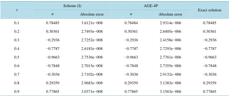
Table 2. The result of the scheme (I) and AGE-4P

(

6 5

)

10 ,n 10 ,T n

τ ₌ − ₌ _{= ∗}τ

.

x

Scheme (I) AGE-4P

Exact solution

u Absolute error u Absolute error

0.1 0.78485 3.6121e−008 0.78484 2.9314e−006 0.78485

0.2 0.30361 2.7493e−008 0.30361 2.6405e−006 0.30361

0.3 −0.2936 2.7252e−008 −0.2936 2.4158e−006 −0.2936

0.4 −0.7787 2.6183e−008 −0.7787 2.7293e−006 −0.7787

0.5 −0.9663 2.7536e−008 −0.9663 2.7761e−006 −0.9663

0.6 −0.7848 2.7015e−008 −0.7848 2.7355e−006 −0.7848

0.7 −0.3036 2.7102e−008 −0.3036 2.9132e−006 −0.3036

0.8 0.29359 2.9683e−008 0.29359 3.1383e−006 0.29359

0.9 0.77865 3.0371e−008 0.77865 3.1563e−006 0.77865

diffusion equations. The methods are _O

(

τ2+_h4

)

accurate and applicable to problems in both Cartesian and polar coordinates. The proposed AGE and AGE-4P methods show superiority. The development of the AGE group methods implies that parallelism can be easily applied advantageously.

References

[1] Celia, M.A., Russell, T.F., Herrera, I. and Ewing, R.E. (1990) An Eulerian-Langrangian Localized Adjoint Method for the Advection-Diffusion Equation. Advances in Water Resources, 13, 187-206.

http://dx.doi.org/10.1016/0309-1708(90)90041-2

[2] Dehgan, M. (2004) Weighted Finite Difference Techniques for the One-Dimensional Advection Diffusion Equation.

Applied Mathematics and Computation, 147, 307-319. http://dx.doi.org/10.1016/0309-1708(90)90041-2

[3] Evans, D.J. and Sahimi, M.S. (1988) The Alternating Group Explicit (AGE) Iterative Method for Solving Parabolic Equations. I: Two-Dimensional Problems. International Journal of Computer Mathematics, 24, 311-341.

http://dx.doi.org/10.1080/00207168808803651

[4] Evans, D.J. and Sahimi, M.S. (1989) The Alternating Group Explicit (AGE) Iterative Method to Solve Parabolic and Hyperbolic Partial Differential Equations. Annual Review of Numerical Fluid Mechanics and Heat Transfer, 2, 283- 389. http://dx.doi.org/10.1615/AnnualRevHeatTransfer.v2.100

[5] Evans, D.J. and Sahimi, M.S. (1990) The Solution of Nonlinear Parabolic Partial Differential Equations by the Alter-nating Group Explicit (AGE) Method. Computer Methods in Applied Mechanics and Engineering, 84, 15-42.

(9)

[6] Evans, D.J. and Sahimi, M.S. (1992) The AGE Solution of the Bi-Harmonic Equation for the Deflection of Uniformly Loaded Square Plate. Report 748, Department of Computer Studies, Loughborough University, Loughborough.

[7] Sahimi, M.S. and Evans, D.J. (1994) The Numerical Solution of a Coupled System of Elliptic Equations Using the AGE Fractional Scheme. International Journal of Computer Mathematics, 50, 65-87.

http://dx.doi.org/10.1080/00207169408804243

[8] Saul. yev V K. (1998) Integration of Techniques for Fluid Dynamics. Springer-Verlag, Berlin.

[9] Kellog, G.R.B. (1964) An Alternating Direction Method for Operator Equations. SIAM Journal on Numerical Analysis,

12, 848-854. http://dx.doi.org/10.1137/0112072

[10] Wang, W.Q. (2002) A Class Alternating Segment Method for Solving Convection-Diffusion Equation. Numerical