Munich Personal RePEc Archive
Identifying behaviour in a multiproduct
oligopoly: Incumbents reaction to tariffs
dismantling
Jaumandreu, Jordi and Moral, Maria Jose
Universidad Carlos III de Madrid
2006
Identifying behaviour in a multiproduct oligopoly:
Incumbents’ reaction to tariffs dismantling
∗
Jordi Jaumandreu
†and Maria J.Moral
‡This version: February 9, 2006
Preliminary
Abstract
The Spanish automobile market of the nineties experienced a perfectly foreseeable
tariffdismantling and a strong demand downturn, with the observed result of an appar-ently sharpened producer competition in products and perhaps in prices. This paper
is aimed at testing whether or not there really was a change in pricing behavior, using
a structural model of competition. To answer that question, we specify, estimate and
test semiparametric pricing equations with panel data for 164 models belonging to the
31firms which competed in the market. The specification includes several equilibriums
as alternative estimating models, considering prominently tacit coalitions by which a
group offirms sets prices, taking into account the cross effects on their demands. The statistical test selects as the best model given the data an unbroken coalition of domestic
and European producers. Comparative results using tight demand side specifications
show that an inadequate specification of the demand side may induce wrong inferences.
∗This paper was completed during the visit of the first author to Harvard University. We are grateful to Simon Anderson and Steve Berry for comments on previous drafts of this paper and to Ariel Pakes for
stimulating thoughts. We also acknowledge useful comments by Tim Bresnahan, Ulrich Doraszelski, Neil
Gandal, Jerry Hausman, Joy Ishii, Marc Ivaldi, Michael Katz, Tor Klette, Pedro Marín, Whitney Newey,
Lars-Hendrik Röller and audiences at the Third CEPR Conference on Applied IO (Bergen), Universidad
Carlos III, Harvard University and EC2 (Marseille). All remaining errors are ours.
†
Dpto. Economía, Universidad Carlos III de Madrid.E-mail: [email protected]
‡
1. Introduction
At the beginning of the nineties, the Spanish automobile market completed a tariff dis-mantling planned since the Adhesion to the EEC. This fact, perfectly foreseeable since years
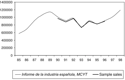
before, complicated with a strong demand downturn (see Figure 1), lead to an apparently
sharpened producer competition, clearly in products and perhaps in prices. Domestic
pro-ducers (installed multinationalfirms) and foreign producers (European and non-European) introduced new models and increased model turnover, engaged in network investment and
high advertising expenditures, while some signs of price competition seemed to appear. This
paper is aimed at testing whether or not there really was a change in pricing behaviour,
using a structural model of oligopolistic multiproduct firms which compete in a product differentiated market.
We understand by behaviour the particular strategies, in a set of well defined market-specific equilibrium concepts, which are sustained at a given moment. Clearly all producers, multiproduct firms with a rough average of more than three car models on the market at any given moment, must be assumed internalizing optimally the cross effects of their model pricing. Moreover, it is natural to assume that firms continuously adjusted model prices to their environment (demand evolution, entry and changes in characteristics of rival models),
independently of the type of pricing equilibrium. The addressed question is whether, in
addition, the environmental changes induced a change infirms’ pricing strategies, modifying their degree of rivalry.
To try an answer to this question, we develop the pricing equation implications of a series
of equilibriums in the form of alternative estimating models. Among these equilibriums
we consider prominently tacit coalitions, by which a group of firms sets prices taking into account the cross effects on their demands, and the change of these coalitions. We then relatively assess the models by testing which one best fits the data.
We specify and estimate the pricing equation with (monthly) panel data on quantity,
to simultaneously test for behaviour and estimate the own and cross elasticities from the
specification, estimation and test of these pricing equations. A key question is how demand side information is treated. We specify price equations free of any restriction on the price
effects coming from functional form demand side constraints, and this turns out to be important for the conclusion. Despite all appearances, our statistical test reveals that
pricing is consistent with an unbroken tacit coordination of domestic and European car
producers and a competitive behaviour on the part of the coming Asian brands. This
conclusion is shown to be perfectly compatible with a broader dynamic game in which all
producers may be competing in product investments (entry, advertising...)
The type of exercise that we perform can have some general interest. We try to uncover
whether a policy change combined with a demand downturn triggered a behavioral change
and which change. A similar issue becomes relevant when any exogenous market event may
trigger a change in behavior: e.g. demand changes, approval of a merger or regulatory
change, irruption of an innovation...As they now stand, quantitative methods of
analy-sis of market competition have largely avoided the question of identifying behaviour and
changes in behavior, with and without government intervention. It seems useful a further
development of techniques to assess the impact of these changes.
Let us briefly comment on the relevant literature. Some of the pioneering works in the “new empirical industrial organization” were motivated by and focussed on the analysis
of behavior changes (Porter,1983; Bresnahan, 19871). More generally, this set out the
question of the precise identification of firms’ behavior2. A detailed specification of a set of market equilibrium behavioral alternative (static) outcomes in a product differentiated market, and the test among them given the data, was carried by Gasmi, Laffont and Vuong (1992). Only a few works have focussed on this type of testing (see for example for a recent
application Jaumandreu and Lorences, 2002), but many discuss the potential effects of different behaviors or use, at some point, alternative behavioral assumptions.
1See also Bresnahan 1981, which develops the model and assess the inpact of imports.
2As something different from the use and empirical measurement of "conjectural variations" (on this use
Exercises of market modelling, concerned with assessing market power and describing its
sources, e.g. product differentiation versus price coordination, discuss the likelihood of dif-ferent behaviors. Nevo 2001, for example, compares the markups implied by his estimated
elasticities, under the alternative behavioral assumptions of Bertrand-Nash competition
and collusion, with the real industry markups, to conclude that pricing is non-collusive and
markups come from product differentiation. Pinkse and Slade 2003 use the estimated elas-ticities to evaluate the effects of real and potential mergers, using the Bertrand equilibrium after concluding that is not rejected by the data. Both examples have in common relying
exclusively on the estimation of demand systems.
On the other hand, two examples of the use of pricing relationships under alternative
be-havioral specifications just come from examples on the automobile market. Berry, Levinsohn and Pakes 1999 estimate their oligopoly model for the American automobile industry under
the three alternative assumptions (to Betrand equilibrium) that firms play Cournot, that there is a "mixed" equilibrium in which Japanese firms set quantities, and that Japanese
firms play Bertrand as do the rest, but colluding among them. Goldberg and Verboven, 20013, in their automobile model for five European countries, also estimate the model under the alternative assumption that firms in the UK collude. The conclusion of these exercises seems atfirst glance somewhat disappointing. The first paper concludes that es-timated parameters are quite similar and that differences seem really do not matter for policy conclusions. The secondfinds the models indistinguishable in terms of fit. However, all estimates of the pricing relationships are carried out constraining markups to have the
value determined by the demand estimated elasticities, either simultaneously (first paper) or even sequentially (second paper) to the demand parameters estimation. As Berry,
Levin-sohn and Pakes 1999 point out, using "the estimated elasticities to investigate the cost side
of the model...would be more flexible and impose less structure..".
More generally, a rich methodology for the specification and estimation of demand in industries with product differentiation has been developed since the papers by Berry,1994, and by Berry, Levinsohn and Pakes,1995. Berry, Levinsohn and Pakes 2004 show in
ular how this methodology may be precise in estimating the patterns of substitution. But
the rich modelling of the demand side has often come at the cost of constraining behavior.
In fact, price relationships have been exploited more as auxiliary equations for demand
identification than as genuine sources of information Here, we explore the extension of ideas and techniques of the recent advances to a framework which addresses the identification of
firms’ behavior through pricing equations.
The methodology consists of specifying and estimate pricing equations which nest the
unobservable marginal cost and the margins established by firms. Margins can be shown to be in general a function of thefirm expected demand price effects, firms’ market shares and behavior. By specifying alternative behaviors, one ends with a series of models which
predict different margins which depend on different ways on observed shares. We derive a semiparametric specification to simultaneously test for behaviour and estimate own and cross elasticities from the price equations, free of constraints imposed by functional form
assumptions on the form of demand. We find that estimation is possible, easy, and gives sensible results. The comparative results using tight demand side specifications show that an inadequate specification of the demand side may induce wrong inferences. By the same reason, the extended practice of doing inferences about market competition using exclusively
demand models can be highly misleading.
The rest of this paper is organized as follows. Section 2 explains in detail the competition
changes that took place in the Spanish market and descriptively explores the price data.
Section 3 discusses the way to specify and test for behavior. Section 4 is devoted to detail
the semiparametric specification and estimation techniques that we apply to the pricing equations, and Section 5 to explain the empirical results. Section 6 concludes. An Appendix
2. Competition changes
At the start of the nineties, the Spanish automobile market4 was served by three types
of car producers: domestic producers, European foreign producers and non-European
for-eign producers, just then beginning to enter the market. The domestic producers were the
multinationals with plants installed in Spain during the seventies and the eighties, aimed at
exporting an important part of production, manufacturing in them some of the car models
they sold5. The European foreign producers were the multinational European producers
without manufacturing in Spanish territory, and the non-European foreign producers were
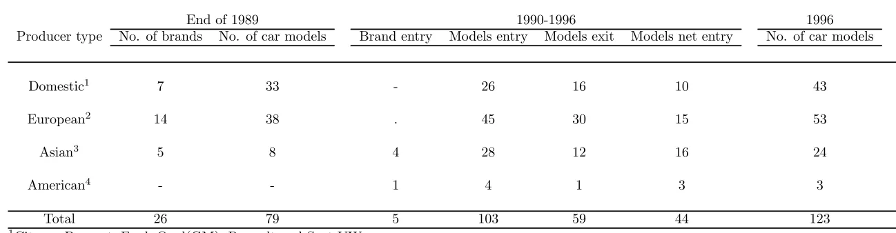
firstly exclusively Asian producers, sometimes possessing an incipient production in Euro-pean territory. Tables 1 and 2 report some basic facts about the structure and evolution of
the market.
Domestic producers accounted for seven brands belonging tofive groups (Citroen-Peugeot, Ford, Opel, Renault and Seat-VW), which coincided with the most important non-Japanese
world producers with the absence of Fiat and Chrysler (recall that Opel is a GM subsidiary).
They had dominated the Spanish market during the eighties, and they started the nineties
with a joint market share of 82% (see Table 1). At this time the European foreign
produc-ers’ supply consisted of 14 brands6, with a joint share of only 16%, but with an important
presence in the upper segments (e.g., more than half of the cars of the highest segment).
And non-European producers accounted initially for 5 Asian brands, representing all
to-gether just a market share of 2%. This number grew up to 9 brands in the following years7,
and the American Chrysler entered the market in 1992.
4The Spanish market was at the time about 1 million cars sold a year, a non-negligible size from the
European perspective.
5In 1990, they sold in the domestic market 39% of the domestic production. Production capacity grew
faster than the market in the following years and, by 1996, the proportion of production going to domestic
sales was only 25%. Notice that Spain was at the time the 3rd European and the 5th World car producer.
6
Audi, Alfa-Romeo, BMW, Fiat, Jaguar, Lada, Lancia, Mercedes, Porshe, Rover, Saab, Skoda, Volvo
and Yugo.
7Honda, Hyundai, Mazda, Nissan, and Toyota were in the market at the start of the 90´s, Mitsubishi
Tariffand non-tariffprotection made it unprofitable to import cars from abroad during the early eighties, dampening even the import of the models from domestic producers not
produced in Spain. All imported cars in 1985 amounted to only 13% of sales. But this
year the Spanish Adhesion Treaty to the EEC, setting the transition framework to full
integration in the single market of 1992, firmly established a different perspective. Tariffs on cars imported from the EEC had to be decreased as stipulated from the then-current
value of 36,7% to zero by the beginning of 1993. And tariffs on cars imported from third countries had to be reduced from the then-current value of 48,9% to the common EEC tariff of 10%.
This perspective immediately started a new competition preparing the coming open
mar-ket, stimulated by a very dynamic demand (see Figure 1). Domestic producers enlarged
the range of models distributed in the market with models imported from their production
in plants abroad, while foreign producers entered new models. Imports had risen to 32%
of sales by 1990 (recall that only 18% are imports by foreign producers) and product
vari-ety was already quite high (79 marketed models, see Table 2). But, the beginning of the
nineties, when tariffs reached the minimum and at a moment in which demand transitorily experienced a stagnation and then a sharp downturn (see Table 1 and Figure 1), seems to
trigger a new competition intensity.
Competition during the nineties adopted several dimensions: product behavior resulted in
a high rate of model introduction and turnover, producers heavily invested in construction
and enlargement of sales networks, engaged in a sharp increase of advertising and seem to
start some price competition which consumers perceived through promotional advertising.
The entry of car models, both replacing old models and introducing in the Spanish market
models absent until this time, was particularly important. In the years following 1990, 104
models entered the market and 59 exited, which implies 123 marketed models by the end of
1996 (see Table 2). Entry was important from the beginning, but notice that exit increases
after the first years (seeTable 1), a sign of more acute product competition8. Asian cars
8
We take as an exit the fact that monthly sales persistently go under some minimun threshold. This can
accounted for a disproportionate share of this entry, but entry by the European foreign
producers and even domestic producers is also important. The role of replacement can be
seen by noting that 90% of exits are separated from a model entry by the same brand by less
than 48 months. Advertising expenditures suddenly jump in 1993, with the expenditure by
unit sold during the period 1993-96 being 170% of the amount during 1990-92.
Among all these competition changes, the focus of this paper is on pricing. In particular,
did the dismantling of tariffs, perhaps complicated with the demand downturn, change
firms’ price behavior? Foreign firms found themselves able to sell at significantly lower prices for the same received prices. Domestic producers experienced the same change for the
models which were introduced from abroad and, at the same time, they expected increased
competition for all their models, including enlarged substitutes and lower rivals’ prices.
All producers are multiproduct firms, with several car models on the market at a given moment, which implies that they must be assumed to optimally internalize the cross effects of their models pricing. Moreover,firms are continuously adjusting each model price to the changing environment (sales level, entry and changes in characteristics), independently of
the game they play. The central question is whether, in addition to all this, the environment
induced any change infirms’ pricing strategies, modifying their degree of rivalry, in the sense explained in the next section.
To acquire an impression of possible pricing behavior changes in our sample period, the
cost changes induced by quality changes must be disentangled. With this aim, we will use
the hedonic coefficients resulting from regressing prices on car characteristics. Let us define the price corrected by quality changes as
e
pjt =pjt−(xjt−xj0)βb (1)
wherexjt is the vector of characteristics of modelj at momentt,xj0 stands for this vector
when the model enters the sample, and bβ represents the cost per unit of characteristic
retire it from sales or some mix of both aspects. Increased exits can be taken in both cases as a sign of
estimated in the hedonic regression9 . Averages of these quality-corrected prices will change
with the entry and exit of models, which embody idiosyncratic qualities that shift the mean.
To correct for these effects, let us define quality change and entry-corrected prices as
e
pt=
1
N
P j
(pejt−(xj0−x)bβ) (2)
where xis the sample mean of attributes and N is the number of models at date t. Entry
and quality change-corrected prices, depicted as indices, give the change in prices which
may be attributed to reasons other than quality-induced cost variations. Of course, they
can show cost changes attributable to other reasons, but they are likely to clearly reflect possible changes in pricing.
Figures 2, 3 and 4 summarize the results of descriptively exploring price changes. Figure
2 represents simple average monthly prices for the three producer types, deflated by the con-sumer price index, and the average received prices; that is, the price received by producers
after deducting the relevant tariffs10. Thefigure highlights an apparent parallel evolution
of European and domestic received prices during the period, at a different level determined by the diverse sales composition, and a sharp decrease of the Asian received prices. Figure
3 represents the evolution of received prices differencing out the quality-induced cost varia-tions (normalized to unity thefirst year), and Figure 4 represents the evolution differencing out the quality composition effects of entry and exit. The hedonic corrections work very well, and in particular denote that quality increments of marketed cars are introduced at
a similar pace for all producers, particularly after 1992, and that Asian entry mainly
con-sists of models directed to compete in the lowest segments as time goes by. Notice how
the sequential corrections notably reduce the range of variation of what remains of prices
variation.
9We employ the coefficients corresponding to one of the estimated models (see section 5), but the exercise
produces very similar results using alternative estimates.
1 0Tariffs during the years 1990, 1991 and 1992 are estimated as 12.37,8.25 and 4.125% for European cars,
and 23.6,18.7,13.8% for non-European cars. Since the beginning of 1993, only remains the 10% tarifffor the
Figure 4 highlights several points. Firstly, all prices tend to show a fall during the first three years (1990-92) and some recovery at some point of the following subperiod. This
suggests partly procyclical pricing, matching the demand evolution reported above, which
does not contradict the possible change in pricing. Secondly, Asian car prices show a sharp
new decrease by the year 1993. Asian producers seem to price more aggressively when the
transitory tariff period reaches its end. These sensible changes in relative pricing (notice that the biggest difference is on average less than 15%) suggests that, since 1993 onwards, the market may be working on a different equilibrium.
3. Testing pricing behaviour with price equations.
This section presents the framework to specify and test for pricing behavior by means of
price equations. Firms are assumed to be multiproduct, competing in a product-differentiated industry given products and their characteristics. Behaviour consists of the particular
strategies, among the set of well-defined equilibrium concepts for price games, sustained by firms. A wide range of behaviours may be covered and the framework is consistent in particular with a broad class of dynamic oligopoly games. The equations stem from market
equilibrium relationships between prices and output represented by shares. Firms’ shares
are hence endogenous variables, given by the relevant (in principle unspecified) demand system. Testing behavior consists of assessing which equilibrium bestfits the data.
3.1 Basic setting.
Let us assume a product-differentiated industry consisting of F multiproductfirms, in-dexed f = 1, ..., F. Each firm produces Jf products and there are in total J = PfJf
products. When we generically refer to a product j, it is implicitly assumed to be one of
the products of the set j = 1, ..., Jf produced by firm f. Demand for each product j is
a function of the J ×1 vector of prices p and all the vectors of products characteristics
x1...xJ. Write demand, for the sake of simplicity, as a function of prices only in the shares
Shares0(p)stands for the fraction of consumers buying nothing. Let sbe theJ×1vector
of shares and define theJ×J price effects matrixD={∂sk
∂pj}, where rowj collects the own
and cross-demand effects of pricej. Product j constant marginal cost, assumed here to be known to simplify notation, iscj11.
3.2 Behaviour.
Assume that prices are strategic complements (reaction curves are upward-sloping)12.
Therefore, any price increase on a product generates a positive externality on the other
product profits, including rival firms’ product profits. It seems simply natural to assume that in any casefirms care about internalizing the cross-price effects of their own profits (they are not “myopic”). That is,firm f sets prices by maximizingPk∈Jf(pk−ck)qk. Butfirms
can also set prices which internalize the positive cross-price effects among a group of rivals. That is, they can form price coalitions (Deneckere and Davidson, 1985), by maximizing
P
k∈Jh(pk−ck)qk, where summation is extended to theJh =
P
f∈hJf products of thefirms
which take part in the coalition13. Let H be the number of coalitions. Belonging to a
coalition implies setting prices to maximize over a set of products which contain the own
products as a subset. Hence, from now on, we will speak exclusively about the grouping
of products at the level of coalition without loss of generality (a situation in which real
coalitions are irrelevant can be thought of as consisting of so many one-member coalitions
asfirms in the market).
Prices maximize profits of the relevant set of products given the other prices, and we will write this as pj = arg max{Pkδjk(pk−ck)qk|δj}, where δj is a 1×J vector of ones and
zeroes, with elementδjk being the indicator of inclusion of productkin the relevant profits
sum (i.e.,δjk= 1ifkbelongs to j0s coalition andδjk= 0otherwise).
1 1The model can be extended to allow for non-constant marginal costs by specifying relevant marginal
cost ascj(1 +k),wherekis the elasticity of cost with respect to output.
1 2With goods being economic substitutes this is the usual case, although it is not the unique possibility.
The model, however, can be extended to any other situation.
1 3
Here we assume thatfirms enter price coalitions with all their products. Other equilibria can be
Let us stack all vectors δj in a J ×J matrix δ. Notice that we are simply specifying
the “one-period” price interactions, not the full conditions for each equilibrium. Pricing
behaviour will be identified without addressing the details of the relevant whole equilib-rium. This allows for a great generality in the equilibriums encompassed. For example,
the particular set of interactions may be the result of a Nash perfect equilibrium under
strategies corresponding to repeated games. In fact, price coalitions are usually understood
as sustainable under repeated games (see, for example, Tirole 1989). The price game can
be also the result of the per-period adjustment of prices in any dynamic oligopoly game of
investment (e.g on advertising or capacity; see, for example, Bajari, Benkard and Levin,
2005). One limitation are dynamic price games, or games in which the prices of one period
impact the demand of future periods. If this situation is thought as the relevant the setting
should be adapted.
3.3 The determination of prices.
With uniproduct Bertrand players or "myopic" multiproduct Bertrand players δ = I.
With multiproduct Bertrand players, each row j has ones in the entries corresponding to
the rest of products produced by the firm that owns j. With price coalitions, the ones of a row expand to all the products of firms in the coalition. The set of FOC conditions which define the price equilibrium corresponding to the relevant behaviour can be written in matrix form as
s+ (δ◦D)(p−c) = 0
where ◦ represents Hadamard product (element by element product). Equilibrium prices
are easily obtained as
p=c−(δ◦D)−1s (3)
System (3) consists of J equations in the form pj = cj +mj(D, δ, s), and shows that
relation-ships, relating the endogenous variables p and s, with s determined additionally through
an arbitrary system of demands. A useful property of equation (3) may be summarized in
the following
Property 1. Product j margin can be written as a linear combination of the shares of
the products included in the coalition, with weights which are a function of the coalition
submatrix of demand price effects. Proof. See Appendix.
A useful implication of this property is that is that δ◦(δ◦D)−1 = (δ◦D)−1.
3.4 Expected price effects.
System (3) could already be the base for testing behaviour14, but it seems reasonnable
and useful to be more specific about the matrixDof price effects. Suppose a market with many differentiated products and consumers heterogeneous in income and tastes who decide among varieties (discrete choice). With M consumers, firm which sets pj will take into
account price effects across the expected quantities E(qk) = P(k)M and hence computes average partial price effects ∂P(k)∂pj . A useful property is the following
Property 2. If each consumer endowed with incomeyand tastes heterogeneityvis
charac-terized by a set of conditional probabilitiesP(j|y, v)of buying the different goods (included the outside alternative), and a change in pricepj changes her probabilities of buying j by
a fraction α(y, pj)15 and varies the rest of probabilities consistently in proportion to their
1 4Equation (3) suggests that behavior can be tested by comparing the
fit of alternative pricing equations,
with behavior imposed on each equation through the constraints on the price derivatives that each equilibrium implies. In addition, an important implication of the above proposition is that, if price effects can be considered stable, and hence estimable, econometric specifications of behavior may be obtained by simply
including the relevant rivals’ shares among the right-hand side variables.
1 5The price effect may be simplified toα(y),butα(y, p
j) is theoretically sounder if we think of the price
relative weights, average market price effects of goodj have the form
E
·
∂P(j)
∂pj ¸
= αjP(j)(1−P(j)) (3)
E
·
∂P(k)
∂pj ¸
= αjP(j)P(k)θjk
where P(j) stand for the aggregate probability that j is bought and αj =α∗j(1 +ωj) and
θjk = (1 +ωjk)/(1 +ωj), with α∗j, ωj and ωjk representing moments computed over the
distribution of consumers heterogeneity (marginal utilities of income and buying probability
covariances respectively). The θjk values are positive and can range from zero to values
well above 1.
Proof. See Appendix.
These market price effects under consumer heterogeneity vaguely remember logit elas-ticities but they differ in two important aspects. Firstly, the α coefficients are product specific. Moment αj is marginal utility of income averaged over the distribution of income
conditioned in choosing j, or “average marginal utility of income for buyers of good j”.
Secondly, cross-price effects are scaled by factors which depend on theω covariance terms. These terms, which measure “proximity” or degree of substitutability of the products, can
be though of as reflecting substitution over the distribution of consumers’ heterogeneity. These aggregate price effects follow by aggregation under arbitrary consumer heterogene-ity. Notice that no parametric assumption is necessary, although parametric demand models
general enough, such as BLP random coefficients model, generate aggregated price effects of this type. BLP techniques estimate these price effects by simulating the unobservable consumer heterogeneity. The interesting thing about price equations is that maximizing
firms can be assumed as computing these average effects from their own knowledge about heterogeneity.
3.5 Price equations.
Property 3.
thatfirms pricing equations can be written as
pj 'cj +
1
αj
[1 +P(j)] +Pk6=jδjk θjk
αk P(k)
Proof. See Appendix.
Under the assumption that aggregated shares converge in probability to aggregated
prob-abilities, we get an equation in terms of observed shares and parameters which are functions
of product-specific average marginal utilities and moments of probabilities over the distri-bution of consumers’ heterogeneity. Modeling cost in terms of observed and unobserved
attributes, adding the time dimension and an error term we then have the price equation
pjt =β0+xjtβ+
1
αj
(1 +sjt) +Pk6=jδjk θjkt
αk
sjt+ξj+ujt (4)
Thefirst two terms of the right hand side model marginal cost in "hedonic" terms (assumex
includes characteristics and squares of characteristics in deviation from their sample means)
while ξ stands for unobserved product-specific costs. The third and fourth terms stand for the margin that the firm would set for product j -given the other prices- in the absence of even multiproduct pricing (myopic behavior). The non-zero terms of the following sum
account for the relevant terms as the result of multiproduct pricing (δjk = 1 when k is
produced by thefirm which producesj)and strategic behavior (δjk= 1whenkis produced
by afirm which prices coordinately with thefirm which producesj).
Equations like (5), representing equilibrium pricing by the firm, are attractive because: a) they do not impose any functional-form structure on the price effects, and b) different be-haviors raise nested models. Unknown coefficientsαandθmay be estimated as coefficients of the shares. Consistent estimation imply the use of IV, because shares are endogenous,
but tests between equilibria may be easily carried out as tests of exclusion restrictions. The
main problem is that we will probably need to estimate a number of parameters which can
be very high, and that the number of parameters increases with the degree of collusion.
from the already likely high lower boundJ. Hence, equations like (4) can only be estimated
for a very small number of products and enough repeated observations for each product j,
either over time or across markets.
The situation partially improves when similar price effects can be assumed for groups of analogous products or “nests.” But any reduction in the dimensionality based on
constrain-ing the price effects tends to cast doubts on the results of the testing of behavior, which relies on evaluating the (own and cross) structure of these effects.
4. Semiparametric specification and estimation.
To overcome the problem of parameter dimensionality we are going to consider a
semi-parametric alternative for equation (5), valid for J large, which avoids imposing strong
previous constraints on the form of the price effects. Notice that α1
j(1 +sjt) can be written as (
1 sjt + 1)
sjt
αj and recall that (alternative) δ
0s
are a-priory specifications representing the behavior we want to test for. We substitute two unknown functions for the two varying-parameter expressions that remain: skt
αk = g(skt)
for all k (i.e. including j =k),and θjkt =θ(djkt), where djk is a measure of the distance
between productskand j,k6=j, in the characteristics space. As the easiest alternative we
are going to use the Euclidean distance.
Equation (5) can now be written as
pjt=β0+xjtβ+ (
1
sjt
+ 1)g(sjt) +Pk6=jδjkθ(djkt)g(skt) +ξj+ujt. (5)
or, to simplify notation, defining conveniently w(djkt) = θ(djkt) if j 6= k and w(djjt) =
(1/sjt+ 1) we can use the more compact form.
pjt =β0+xjtβ+Pkδjkw(djkt)g(skt) +ξj +ujt. (6)
Model (6-7) is a semiparametric equation which includes two interacted unknown functions,
each one with its own economic interpretation. To estimate them we are going to use
multivariate unknown functions16 We are going to specifyg(s
k) =ρ0+ P
iρisikand impose
positivity on the θ effects by specifying θ(djk) = exp(λ0+Piλidijk).Notice that the fact
that the g(.) function appears in (6) multiplied by a known factor and that both functions
are interacted allows in principle for the identification of the constants separately toβ0.
With both series estimators having the same number of termsI, the number of parameters
to be estimated by reason of the unknown functions are2I.Identification can be intuitively though of in the following way. Approximate θ(.) by the sum of a constant and terms in
powers of d.The product of this approximation ofθ(.) by g(.) is, for a given termk of the
sum, a polynomial including the tensor product of the powers of dands.The sum of these
polynomials across k, gives a new polynomial in terms of sums of products of powers of d
andsacross goods. This polynomial would constitute an identifiable linear model on whose coefficients we are in fact imposing nonlinear constraints.
Estimation can be carried out by means of a nonparametric two stage least squares
method (Newey and Powell, 2003). We use the version of Ai and Chen (2003) or "sieve
minimum distance" estimator. We proceed as follows. Dummies for each one of the models
to account for thefixed effects and the other parameters which enter linearly (time dummies, characteristics and the squares of characteristics) are "concentrated out". This leaves us
with a search for the parameters of the two unknown functions. We set the problem as a
nonlinear GMM problem where we use as instruments all the variables which enter linearly
and all the sums of the products of powers of the variables on which we want to condition
dand s(i.e. the terms of the "aggregate" polynomial). We consider the distance between
products as exogenous and hence we use it as instrument. And we use as instrumentslagged
six months to avoid the possible correlation of more contemporaneous values with the error
term of the equation. The sums are computed across all competitors, independently of the
particular competition model represented byδ,to keep instruments the same increasing the
comparability of the estimates.
Both functions are specified as cubic polynomials and, while g(.) is kept totally unre-stricted, we impose (decreasing) monotonicity on the θ(.) function. Trials have included
the estimation without "fixed effects," the use of higher order polynomials, the employ of different lags of s and the use more instruments. It seems to be important to estimate including fixed effects and assuming the endogeneity ofs, but the change in other details seem to change little.
The model is estimated for different pre-specified behaviors embodied through theδspecification. The semiparametric specification has transformed the problem however in a series of non-nested estimates which use different regressors. The testing of the models against each other is then carried out by means of the Lavergne-Vuong (1996) test for selection of regressors in
nonparametric estimation when models are non-nested. The Lavergne-Vuong test compares
the MSE of each two models taking into account the variance of the difference between the MSE’s of the two estimates.
5. Empirical results.
We estimate price equations using data on the car models sold on the Spanish market
from 1990 to 1996 by the 31firms with a presence in the marketplace. The data consist of unbalanced panel observations for a rather standard number of individuals (164 models17)
but with the more unusual characteristic of monthly data frequency (which gives a maximum
of 84 observations per individual). Using the price equilibrium relationships established in
Section 3, and the semiparametric specification and techniques described in Section 4, the
final objective of this empirical exercise is to obtain estimates under the assumption of different behaviours and to test their relative likelihood given the market data. This section begins giving some details on the employed variables and equilibrium concepts, goes on
some detail in explaining the results of estimating the semiparametric equations andfinally compares the estimates with the results obtained with other specifications.
1 7
The total number of models are 182, but we must drop 18 in estimation due to the lack of enough lagged
observations: the 16 entrant models of the last year and 2 models which stayed in the market less that 12
5.1 Variables and equilibriums.
Our dependent variable pjtis producer received prices or observed prices once deducted
the tariff, i.e. pob
jt/(1 +tariffjt)We must carry out the simultaneous estimation of a nested
marginal cost function and the firms’ markups. To estimate marginal costs, we adopt the “hedonic” approach18: we take cost as a function of a set of product attributes. Specifically,
we approximate marginal cost around its mean using a quadratic polynomial with attributes
entering in the form of deviations with respect to the sample mean and the squares of these
deviations. We specify marginal cost as independent of output (in fact we do not observe the
relevant output for most of the involved producers), we include an estimate of the relevant
average unit labour costs for each producer and we allow for unobserved components of
marginal cost.by adding the unobservable model-specific effect.
The employed attributes are the power measureratio cubic centimeters to weight(CC/Weight),
the fuel efficiency ratio km to liter (Km/l), used in the particular form of the relative
ef-ficiency in city driving with respect to 90 Km/h driving, the measure of size and safety length times width (Size), the maximum speed in km/h (Maxspeed) and the materials use
indicator weight (Weight)19 The use of other characteristics or a more complete list does
not change the main results.
We estimate the measure djk of “distance” or degree of substitutability between each
two products using the four first attributes. Let xj and xk represent the relevant vector
of characteristics, distance is computed as djk = £(xj−xk)0Σ−1(xj −xk) ¤1/2
, where Σ
represents the matrix of empirical sample covariances.
Equations are estimated forfive pre-specified behaviors: myopic; Betrand multiproduct; a price coalition sustained by the domestic and Europeanfirms; the break up of this coalition in 1993 reverting to Bertrand; and full collusion. The first behaviour is taken into account
1 8Cost estimates starting from regressions on product characteristics can be called “hedonic” because they
use the methodology of the traditional hedonic price regressions (see Griliches,1961; Rosen, 1974, and the
recent discussion in Pakes, 2003). We follow the approach by Berry, Levinsohn and Pakes (1995).
1 9We try to be deliberately close to Berry, Levinsohn and Pakes’ (1995) speci
fication for the sake of
as an unlikely lower bound. The second implies that behaviour was Bertrand-Nash all the
time and for all players, a common assumption in many models and estimates of this type.
The third makes the sensible assumption that domestic and European producers set prices
internalizing the cross effects of their prices; i.e., they constitute a price coalition while Asian producers are assumed to play Bertrand. The fourth assumes that this coalition broke up
at the end of 1992,.with the Domestic and European producers switching to play Bertrand.
Thefifth makes the unrealistic assumption that behavior was collusion of all players all the time.
5.2 Results from semiparametric equations.
Table 3 shows the estimates of the pricing equations under the different behavior spec-ifications. Table 4 shows the results of the Lavergne-Vuong test for model selection. The model representing an unbroken price coalition is clearly the closest to the data. Next
sub-section shows the degree of coincidence of this conclusion with the estimates obtained by
other methods, what turns out to be a robustness check which reinforces the interest of the
estimates. Let first explore with some detail the results of the estimate.
The most natural product of the selected model is the estimation of margins. Let us study
the implied margins and the corresponding elasticities. Despite many efforts to avoid the problem, the g(.) function estimate remains negative for the preferred model at somewhat
less than 12% of the data, mainly in the right tail (big svalues). As some negative values
for theg(.) function can be perfectly consistent with our "fixed effects" specification (both the constant and the effects can be picking up some specific margin intercepts) we take into account part of them. Specifically, we define a trimmed estimatorbgby setting the 5% lower values (all in the right tail) to the (still negative) value of the function at this percentile.
Then we compute margins as(s1
j + 1)gb(sj) +
P
k6=jδjkbθ(djk)bg(sk),and set to zero the small
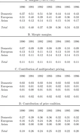
proportion of margins which result negative (2.4%). Panel A of Table 3 shows the estimated
margins and their evolution for the whole sample and for competitors grouped in domestic,
margins into a part explained by Bertrand pricing, a part added by thefirms’ multiproduct optimal pricing, and the part explained by price coordination. It must be taken into account
that this decomposition is done given the other prices.
The selected model allows also us to estimate the own and cross elasticities consistent with
these margins. The own elasticities can be estimated asbηj =−αbj(1−sj)pj '−pj/mbj and
the cross-elasticities as bηjk = αbjsjpjbθjk '(pj/mbj)1−sjsjbθjk, where mb is an estimate of the
myopic margins.We start with the estimatorme = (s1
j+1)(bg+|minbg|).As we have, however,
some margins estimated very close to zero and others set to zero part of the elasticities take
high (absolute) values and (minus) infinity respectively. To avoid this we use a trimmed version (Newey, 1994) defined as follows
b
m(me) =
b if me = 0
b
·
1 +³2bme´2
¸
if 0<me ≤2b
e
m >2b
Asbapproaches to zero some elasticities grow arbitrarily large. As the important insight is
the structure of elasticicities, which remains almost invariant to changes in their absolute
value, we choose a value to obtain rather conventional elasticity values (b= 0.01).
Table 6 shows averages of the estimated elasticities grouped by standard automobile
segments. Notice the important variation of the cross elasticities (next section shows that
this variation is more important by far than with the estimates obtained with any other
estimator). Recall that the value of cross-elasticities is governed by the estimated thetas,
representing covariances of buying probabilities over the heterogeneity of consumers, which
measure the intensity of cross price effects between two given car models . Table 7 shows than an average model gets a relatively intense competition of 30% of the competitor car
models (θ >1)and relatively weak competition from the other 70%. It would be interesting
to develop some examples for particular car model cases. Table 8 give average values for the
thetas, which can be taken as measures of the intensity of competition inside of the employed
groupings in doing the table (values in the diagonal) and between cross segments (of-diagonal
has some content.
5.3 Results from other specifications.
The same problem with the same sample was subjected to three other alternative
es-timation procedures. Firstly, we used completely parametrized price equations consistent
with a nested logit specification of demand. Nests were defined according to the conven-tional automobile segments mentioned above, the model was flexibilized by allowing the price parameters to vary by segments, and the degree of correlation inside nests was given a
standard value. Secondly, we estimated a nonlinear system consisting of the nested logit
de-mand equation corresponding to the previous model and the corresponding price equations,
imposing the cross equation constraints. Thirdly, we estimated the nonlinear system
con-sisting of a random coefficients utility model with its corresponding price equations (BLP estimation). Shares and the share derivatives are here obtained by simulating the
con-sumers’ income distribution and the random shocks interacted with characteristics. These
estimates can be seen as an ordering of demand specifications ranked in ascending order of
flexibility.
All three models are parametric and equilibriums are non-nested, so we used the Rivers
and Vuong (2002) test for selection among (possibly misspecified) nonnested models, in the version in which the selection criteria is based on the value of the objective function
which has been minimized (the GMM objective); i.e. the value T = √σbn(Q1 −Q2) to be
compared with critical values of aN(0,1), with bσ an estimate of the sampling variance of the difference between objectives. Values of the "first-step" objective function are used, which employ the same consistent estimator of the weighting matrixA, based on the same
set of instruments for the series of models to be compared. Variance is taken as
σ= 4hG01AE11AG1+G 0
2AE22AG2−2G 0
1AE12AG2 i
and estimated usingGbi = 1nPm1(bγ) and Eb12= n1P m1(bγ)m2(bγ)0.
Table 9 reports the result of testing behaviour with these estimation procedures. In
The second estimation procedure gives Bertrand for all players and time periods as the
best equilibrium. The third procedure (BLP estimation) gives the same result the our
semiparametric estimation, pointing out the price coalition as the model that best fits the observe data. This result seems however not to be robust to all kind of instruments and
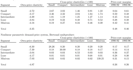
tends to assign also a too good score to collusion. Table 10 gives the estimated averages
of elasticities in the second and third estimation procedures, to be compared with the
averages in Table 6. Acceptation or rejection of equlibriums can be in fact traced back to
the estimation of the level and structure of these elasticities.
6. Conclusion.
This paper has addressed the question of whether the Spanish car market underwent
a change in pricing behavior that coincided with the tariffs dismantling attained by 1992. The answer is no, despite that the the simple observation of the data can induce to
be-lieve a change in behaviour. Careful specification of pricing equations, and their estimation by semiparametric methods, has allowed us to point out that tacit coordination in pricing
maintained up to this moment by domestic and European producers is likely to have
con-tinued, given the data, versus the alternative hypothesis that this coordination broken up
by this time. The specification and estimation of a random coefficients utility model and its corresponding pricing equations gives the same result. One caveat, however, is in order:
this can be only one part of the whole picture. One advantage of our framework is that
is consistent with the likely pricing of more complex dynamic competition models. The
corresponding disadvantage is that we cannot say anything about the rest of the setting.
For example, coordination in prices is likely to have been kept at the same time that was
an increased competition in advertising and the building of sales networks. But the
an-swer provides, at least, afirst step for focussing on broader hypotheses and more complex structural models.
More generally, a lesson of this study is that to specify semiparametric price equations,
behavior, is possible, easy and useful. The model is identified and gives sensible results. The estimation amounts to solve a nonlinear GMM problem. The model provides estimates
of margins and elasticities free of parametric demand side assumptions and permits to
decide which behavior is closest to the market data as well as to base the estimates on this
behavior specification. The estimated margins can be used to do welfare analysis and for policy recommendations. The comparative results using tight demand side specifications show that an inadequate specification of the demand side may induce wrong inferences. In fact, all comparisons show that demand specifications seem to constitute a potential source of bias to be taken seriously into account. By the same reason, the extended practice of
doing inferences about market competition using exclusively demand models can be highly
misleading. One interesting avenue for future research is how to integrate more demand
Appendix
Proof of Property 1.
To see this property, letPHbe the permutation matrix which induces a re-ordering offirms
(and hence products) according to the coalition they belong to. PHs+PH(δ◦D)PH0 PH(p− c) = 0 is a system equivalent to (3), and hence PHp =PHc−(PH(δ◦D)PH0 )−1PHsgives
the same prices. But, by definition of δ,(PH(δ◦D)PH0 )−1 is a block diagonal matrix.
Proof of Property 2.
Consumers are endowed with income y and unobservable heterogeneity v, .and y and
v are distributed independent with densities f(y) and g(v). Marginal utility of income is
modelled as depending only ony for simplicity, generalization toα(y, pj)is straightforward
and important; heterogeneityvis associated to a unique characteristicr again for simplicity,
and the independence assumption could be also relaxed.
LetP(j)be aggregate probability of buying goodj, andP(j|y, v)probability conditional
on (y, v).For simplicity of notation we are systematically omitting x and p from the
con-ditioning set. Note also that probabilities are conditional expectations. A more complete
notation would be to writeP(j|y, v) asE[ζj = 1|x, p, y, v].
P(j) =R P(j|y, v)f(y)g(v)dydv
A natural object of interest are average partial effects, namely average price effects ∂P(k)∂p
j .
Assuming that integral and derivative can be interchanged,
∂P(k)
∂pj
= E
·
∂P(k|y, v)
∂pj ¸
=R ∂P(k|y, v)
∂pj
f(y)g(v)dydv
= Rα(y)P(j|y, v)P(k|y, v)f(y)g(v)dydv
= Rα(y)£RP(j|y, v)P(k|y, v)g(v)dv¤f(y)dy
where the third equality comes from the assumption on consumer probability changes The
term between brackets can be written as
where P(j|y) = RP(j|y, v)g(v)dv is probability of buying j for given y averaged over the distribution of v, and the second term is Covv[P(j|y, v), P(k|y, v)] for a given y over the
distribution of v. We are unable to write analytically P(j|y) but we know that it is the
right probability by the Law of Iterated Expectations. Using this and then writing thefirst term in a similar way we have
∂P(k)
∂pj
= Rα(y)P(j|y)P(k|y)f(y)dy+R α(y)Covv[P(j|y, v), P(k|y, v)]f(y)dy
= αjP(j)P(k) +Covy[α(y)P(j|y), P(k|y)]
+R α(y)Covv[P(j|y, v)P(k|y, v)]f(y)dy
whereαj =R α(y)f(y|j)dy .
Bayes rule is used to write Rα(y)P(j|y)f(y)dy as£R α(y)f(y|j)dy¤P(j) =αjP(j).
Mo-mentαj is marginal utility of income averaged over the distribution of income conditioned
in choosing j, or “average marginal utility of income for buyers of good j”.
Average price effects turn therefore out to be decomposable into one part which depends on average marginal utility and average probabilities and another which depends on
covari-ance moments over the distribution of heterogeneity. As a convenient way to express the
total effects, dividing and multiplying byαjP(j)P(k)we can write
∂P(k)
∂pj
=αjP(j)P(k)(1 +ωjk)
whereωjkdepends on covariance moments of the probabilities of buyingjandkover the
dis-tribution of consumers’ heterogeneity. Similarly, we can write∂P(j)∂p
j =−αjP(j) [1−P(j)] (1+
ωj).It is easy to check that ωj =Pk6=j P(k)
1−P(j)ωjk, which ensures the additive properties of
price effects.
Proof of Property 3.
LetαandP beJ-dimensional diagonal matrices collecting theαj and theP(j)’s
respec-tively; define the matrices W = [1 +ωjk]andIW =diag(W); and letp and c be theJ×1
vectors of prices and costs andea J×1vector of ones. The set ofJ FOC conditions may
P e−[δ◦(αP IW −αP W P)] (p−c) = 0
and taking into account that element by element product ofδby any diagonal matrix leaves
the matrix unchanged, it is easy to arrive at the expression
p=c+£I−δ◦(IW−1W P)¤−1IW−1α−1e
Elements of rowjof matrix(IW−1W P)add upP(j) +1+ω1
j
P
k6=j(1 +ωjk)P(k)and taking
into account the restriction on the ωj’s it can be shown that this sum is [ P
kP(k)]+ωj
1+ωj <1.
Maximum row sum matrix norm|||δ◦IW−1W P|||row <1and hence £I −δ◦(IW−1W P) ¤−1
=
(I +δ◦IW−1W P + (δ◦IW−1W P)2 +...), (Horn and Johnson 1985, Theorem 5.6.15).
Ne-glecting the squared and following terms, which depend on the square of probabilities, and
substituting into the previous equation we get
p'c+ (IW−1+δ◦IW−1W P IW−1)α−1e
or, developing the expression for price pj
pj 'cj+
1
αj(1 +ωj)
[1 +P(j)] +Pk6=jδjk
1 +ωjk αk(1 +ωj)(1 +ωk)
References
Ai, C. and Chen, X. (2003), Efficient estimation of models with conditional moment re-strictions containing unknown functions, Econometrica, 71, 1975-1843.
Bajari, P., L.Benkard and J. Levin (2005), “Estimating dynamic models of imperfect
competition,” mimeo, Stanford University.
Berry, S.T. (1994),“Estimating discrete-choice models of product differentiation,” RAND Journal of Economics, 25, 2, 242-262.
Berry, S.T., J. Levinsohn and A. Pakes (1995), “Automobile prices in market equilibrium,”
Econometrica, 63, 4, 841-890.
Berry, S.T., J. Levinsohn and A. Pakes (1999), “Voluntary export restraints on
automo-biles: evaluating a trade policy,” American Economic Review, 89, 400-430.
Berry, S.T., J. Levinsohn and A. Pakes (2004), “Differentiated products demand systems from a combination of micro and macro data: the new car market,” Journal of Political
Economy, 112, 1, 68-105.
Bresnahan, T.F. (1981), “Departures from marginal-cost pricing in the American
automo-bile industry,” Journal of Econometrics, 201-227.
Bresnahan, T.F. (1987), “Competition and collusion in the American automobile industry:
The 1955 price war,” Journal of Industrial Economics, 35, 4, 457-82.
Bresnahan, T.F. (1989), Empirical studies of industries with market power, in R. Schmalensee
and R.Willig (eds.), Handbook of Industrial Organization, North-Holland.
Deneckere, R. and C. Davidson (1985), “Incentives to form coalitions with Bertrand
com-petition,” Rand Journal of Economics, 4, 473-486.
Goldberg, P.K. (1995), “Product differentiation and oligopoly in international markets: the case of the U.S. automobile industry,” Econometrica, 63, 4, 891-951.
Goldberg, P.K. and F. Verboven (2001), “The evolution of price dispersion in the European
car market,” Review of Economic Studies, 68, 811-848.
Griliches, Z. (1961), “Hedonic price indexes for automobiles: An econometric analysis of
quality change,” reprinted in Z. Griliches (Ed.) “Price Indexes and Quality Changes,”
Harvard University Press.
Horn, R. and C. Johnson (1999), Matrix Analysis, Cambridge University Press.
Jaumandreu, J. and J. Lorences (2002), “Modelling price competition across many markets
(An application to the Spanish loans market),” European Economic Review, 46, 1,
93-115.
Lavergne, P. and Q. Vuong (1996), “Nonparametric selection of regressors: The nonnested
case,” Econometrica, 64, 207-219.
Nevo, A. (2001), “Measuring market power in the ready-to-eat cereal industry,”
Econo-metrica, 69, 307-342.
Newey, W. (1994), “Series estimation of regression functionals,” Econometric Theory, 10,
1-28.
Newey,W. and J. Powell (2003), “Instrumental variable estimation of nonparametric
mod-els,” Econometrica, 71, 1565-1578.
Pakes, A. (2003), “A reconsideration of hedonic price indexes with an application to PC’s,”
American Economic Review, 93,5 1578-1596.
Pinkse, J. and M. Slade (2003), “Mergers, brand competition, and the price of a pint,”
European Economic Review, 48, 617-643.
Rivers, D. and Q. Vuong (2002), “Model selection tests for nonlinear dynamic models,”
Econometrics Journal, 5, 1-39.
Rosen, S. (1974), “Hedonic price and implicit markets: product differentiation in pure competition,” Journal of Political Economy, 82, 34-55.
Table 1
The Spanish car market in the 90s: basic statistics
Share of [Of which Share of Share of
Year Sales Sales Models Models No. of domestic imported European Asian
index entry exit models1 producers2 cars] producers2 producers2
1990 971,466 100.0 19 2 96 82.0 [14.3] 16.0 2.0
1991 878,594 90.4 10 3 103 80.0 [13.7] 16.9 3.1
1992 973,414 100.2 16 7 112 81.3 [14.3] 14.6 3.9
1993 735,993 75.8 12 8 116 80.7 [19.1] 13.9 5.2
1994 897,492 92.4 13 13 116 78.6 [16.2] 15.8 5.3
1995 822,593 84.7 17 12 121 77.0 [15.2] 15.7 6.8
1996 897,906 92.4 16 14 123 75.0 [15.2] 15.8 8.4
1At the end of the year.
Table 2
The Spanish car market in the 90’s: competitors, brands and model entry and exit
End of 1989 1990-1996 1996
Producer type No. of brands No. of car models Brand entry Models entry Models exit Models net entry No. of car models
Domestic1
7 33 - 26 16 10 43
European2
14 38 . 45 30 15 53
Asian3
5 8 4 28 12 16 24
American4
- - 1 4 1 3 3
Total 26 79 5 103 59 44 123
1
Citroen-Peugeot, Ford, Opel(GM), Renault and Seat-VW
2
Audi, Alfa-Romeo, BMW,Fiat, Jaguar, Lada, Lancia, Mercedes, Porshe, Rover, Saab, Skoda, Volvo and Yugo.
3
Honda, Hyundai,Mazda,Nissan and Toyota before 1990; Mitsubishi, Suzuki, Subaru and Daewo since 1990 and after.
4
Table 3
Preliminary results from the estimation of semiparametric pricing equations
Dependent variable: pjt/(1 +τjt)
No. of car models: 164; Sample period1: 1991-96; No. of observations1: 7,122
Estimation method: Nonparametic two stage least squares
Behavior Myopic pricing Betrand multiproduct Price coalition Coalition breaks up 1993 Collusion
Variable Parameter SE Parameter SE Parameter SE Parameter SE Parameter SE
Constant -2 - 0.24 1.207 1.907 0.529 2.638 0.168 1.505 0.618
Unit labor costs 0.126 0.169 -0.132 0.333 0.138 0.220 0.027 0.322 0.263 0.404
CC/Weight -0.191 0.346 1.299 0.647 -0.029 0.148 0.255 0.291 0.016 0.372
Maxspeed 2.569 0.404 2.133 0.519 1.834 0.359 2.391 0.662 1.991 0.683
Km/l 0.549 0.099 -0.040 0.159 0.204 0.109 0.554 0.280 0.128 0.265
Size 1.555 2.728 -6.496 2.786 0.017 1.337 -0.006 1.090 -0.473 1.602
Weight -1.254 0.394 0.472 0.800 -0.729 0.481 -0.715 0.582 -0.407 0.615
(CC/Weight)2 0.239 0.098 0.381 0.120 0.410 0.130 0.218 0.191 0.550 0.189
(Maxspeed)2 3.580 0.552 5.725 1.149 5.046 0.755 4.323 0.466 5.486 0.702
(Km/l)2 -2.278 0.349 -0.573 0.391 0.102 0.232 0.362 0.358 0.572 0.524
(Size)2 4.124 8.477 28.142 10.519 9.507 5.047 5.835 2.705 10.330 5.125
Yearly dummies yes yes yes yes yes
Model dummies yes yes yes yes yes
g(s)function yes yes yes yes yes
θ(d)function no yes yes yes yes
MSE 1.6437 0.9075 0.3849 0.7459 0.4662
1Total sample period and observations are 1990-96 and 9,090 respectively.
Table 4
Testing behavior with the semiparametric price equations1,2
Bertrand multiproduct Price coalition Coalition breaks up 1993 Collusion
Myopic 2.43 3.85 2.73 3.63
Bertrand multiproduct 9.62 2.14 7.19
Price coalition -6.93 -2.64
Coalition breaks up 1993 6.14
1
Lavergne-Vuong test for nonparametric selection of nonnested regressors: T = √bσn(M SErow−M SEcol)to be compared with aN(0,1). 2
Table 5
Average margin evolution 1990-1997 by producers, as predicted by selected model, and decomposition
A. Margins (=B+C+D).
1990 1991 1992 1993 1994 1995 1996
Domestic 0.37 0.51 0.51 0.50 0.44 0.44 0.43 European 0.31 0.40 0.39 0.41 0.40 0.36 0.33 Asian 0.13 0.12 0.14 0.15 0.15 0.16 0.17
Total 0.31 0.40 0.37 0.39 0.36 0.34 0.33
B. Myopic margins.
1990 1991 1992 1993 1994 1995 1996
Domestic 0.07 0.09 0.09 0.08 0.09 0.10 0.09 European 0.13 0.13 0.11 0.13 0.13 0.10 0.10 Asian 0.12 0.11 0.12 0.14 0.13 0.14 0.15
Total 0.11 0.11 0.11 0.11 0.11 0.10 0.11
C. Contribution of multiproduct pricing.
1990 1991 1992 1993 1994 1995 1996
Domestic 0.02 0.03 0.02 0.04 0.02 0.02 0.02 European 0.01 0.01 0.02 0.01 0.02 0.01 0.01 Asian 0.01 0.00 0.01 0.01 0.01 0.01 0.02
Total 0.01 0.02 0.01 0.02 0.02 0.02 0.01
D. Contribution of price coalition.
1990 1991 1992 1993 1994 1995 1996
Domestic 0.27 0.39 0.36 0.36 0.32 0.31 0.32 European 0.16 0.25 0.24 0.26 0.25 0.24 0.21 Asian 0.00 0.00 0.00 0.00 0.00 0.00 0.00
Table 6
Average own/cross-price elasticities (by segments) with semiparametric price equation
Cross-price elasticities (×100)
Segment Own-price elasticity Small Compact Intermediate Luxe Minivan
Small -10.12 7.47 4.86 2.65 1.20 1.69
Compact -11.01 3.54 6.86 5.46 2.52 2.00
Intermediate -4.22 0.44 1.04 1.16 0.64 0.38
Luxe -2.04 0.01 0.02 0.04 0.04 0.01
Minivan -1.6 0.01 0.01 0.01 0.01 0.03
Total -5.78
Table 7
The distribution of theta values Theta value Percentage of observations
θ≤0.50 45.4
0.50< θ≤1 24.6
1< θ≤2 19.5
[image:37.612.116.430.408.522.2]2< θ 10.5
Table 8
Average estimated theta values (by segments)
Theta values
Segment Small Compact Intermediate Luxe Minivan
Small 1.68 0.89 0.50 0.25 0.41
Compact 0.89 1.59 1.28 0.63 0.51
Intermediate 0.50 1.28 1.46 0.98 0.55
Luxe 0.25 0.63 0.98 1.01 0.40
Table 9
Behavior selected by other estimators1
Estimator Behavior
Parametrized (nested logit) price equations Coalition breaks up in 1993 Nonlinear parametric (nested logit) demand-price system Bertrand multipoduct Nonlinear system with simulation (random coefficients or BLP estimation) Price coalition
1
Table 10
Average own/cross-price elasticities and margins by segments with other estimators
Nonlinear system with simulation (random coeffcients or BLP estimation), Price coalition:
Cross-price elasticities (×100) Price-cost margins
Segment Own-price elasticity Small Compact Intermediate Luxe Minivan 1990-92 1993-96
Small -2.72 2.67 2.02 1.46 0.91 1.22 0.64 0.61
Compact -3.17 2.46 2.32 2.04 1.64 1.74 0.50 0.48
Intermediate -3.39 1.01 1.19 1.25 1.27 1.14 0.45 0.44
Luxe -3.84 0.19 0.33 0.48 0.71 0.52 0.38 0.38
Minivan -3.16 0.19 0.27 0.34 0.46 0.39 0.42 0.41
Total -3.35 0.48 0.46
Nonlinear parametric demand-price system, Bertrand multproduct:
Cross-price elasticities (×100) Price-cost margins
Segment Own-price elasticity Small Compact Intermediate Luxe Minivan 1990-92 1993-96
Small -6.30 28.26 0.20 0.20 0.20 0.20 0.17 0.17
Compact -7.39 0.18 30.09 0.18 0.18 0.17 0.14 0.14
Intermediate -3.04 0.03 0.03 6.53 0.03 0.03 0.36 0.37
Luxe -4.17 0.01 0.01 0.01 9.68 0.01 0.28 0.30
Minivan -7.03 0.02 0.02 0.02 0.02 139.25 0.31 0.15
Figure 1
Sales evolution in the Spanish car market
0 200000 400000 600000 800000 1000000 1200000 1400000
85 86 87 88 89 90 91 92 93 94 95 96 97 98