Munich Personal RePEc Archive
School Competition
Jaag, Christian
2006
School Competition
Christian Jaag
∗January 4, 2006
Abstract
This paper considers the influence of spatial competition on education and its effect on students’ school choice and educational achievement by explicitely modeling educational production and the students’ participation decision. Education at school is a function of teacher effort and class size. Students decide which school to attend on the basis of an assessment of the associated costs and prospective benefits from doing so. We analyze how competition between schools affects equilibrium resource spending and school diversity as well as the level and distribution of student attainment and welfare. The consideration of spatial aspects of school choice without recourse to vertical differentiation is a unique contribution of this paper.
We argue that schools in metropolitan areas with short ways to school and many potential students face fiercer competition which increases school productivity and student performance. This result confirms the findings in Hoxby (2000). Overall learning time in school is constant in the probabil-ity that students behave well if students are segregated by type. However, better behaved students have a higher achievement due to higher optimum resource spending.
Finally, we support our argument by an empirical analysis of student per-formance in various matura schools in Switzerland.
∗Institiute of Public Finance and Fiscal Law, University of St.Gallen, Varnb ¨uelstrasse 19, CH-9000
St.Gallen,christian.jaag@unisg.ch. Financial support from the Swiss National Science Foundation
1
Introduction
Competition between schools is one of the most hotly debated approaches to providing incentives in order to improve education. The first step towards a competitive environment for schools is the introduction ofschool choice. In such a system, public schools have to compete at least against other public schools. A second step is the introduction ofvouchersto enable students to attend any school – public or private – they (or their parents) like. The best-known proponent of this idea is Friedman (1997). Distinguishing between the financing and the pro-vision of education, it is possible to assess whether private schools perform bet-ter than public schools. Vouchers create a market in education by establishing an exchange mechanism and the price is the nominal value of the voucher. As an entitlement to an amount of schooling, such vouchers may allow students to choose their education, where – because of government funding – the inequali-ties which potentially arise with choice are ameliorated. Potential consequences of voucher programs include changes in who enters the teaching profession, how teachers and students allocate time and effort to various tasks, and how students sort themselves into schools, classrooms, and neighborhoods (cf. Neal, 2002).
Evidence concerning the market for education suggests that there are beneficial effects from vouchers and school choice, but up to now, research can not give clear answers to the basic questions whether and how competition leads to better school performance. In this paper, we focus on the implications of school district properties and schooling policy measures for student attainment and achieve-ment.
performance is prohibited. In the empirical application of the model we concen-trate on the upper secondary level of education since this is the one on which students are most mobile and the establishment of free school choice and compe-tition is explicitly intended to provide schools incentives to improve. Geograph-ical restrictions for attending certain schools being very diverse throughout the country, an important focus of the paper is on the impact of the geographical dimension on school competition and student attainment.
We first present an overview of the literature on school competition. Then, we provide a theoretical framework for the analysis of the effects of school district properties and policy measures on student attainment and achievement. Finally, we discuss the actual competitive environment for matura schools in Switzer-land and assess parts of our theoretical findings with data from the Program for International Student Assessment (PISA) in the context of the Swiss school sys-tem.
2
Related Literature
A large body of theoretical research examines the effects of competition on school quality and sorting across schools, cf. eg. Epple and Romano (1998, 2002), Hoyt and Lee (1998), Nechyba (1996, 1999, 2000), Caucutt (2002), and McMillan (2004). In this research, schools are often treated as passive technologies converting re-sources into educational achievement, thus abstracting from institutional char-acteristics of the school system and potential incentive effects of vouchers that influence school efficiency. Empirical findings on the effectiveness of competi-tion between schools are controversial. Among the proponents of school choice are West (1997), Hoxby (2000, 2003), Holmes, DeSimone, and Rupp (2003); rather critical is Carnoy (1997). The potential problem of decreased equity in competi-tive school systems, where private schools tend to privilege certain student types, is addressed in Ambler (1994) and Ladd (2002).
given to quantifiable examination results than to what is important. Thus, the costs of a voucher system may outweigh the expected benefits of introducing competitive pressure to schools and greater freedom into the provision of educa-tion.
3
The Model
3.1
Model Outline
We develop a theoretical model which focuses on the effect of vouchers with respect to a school’s choice of spending on schooling resources and class size and students’ participation decision if education is compulsory. The main differ-ence to the literature lies in the use of a more elaborate educational production function and the explicit modeling of students’ participation decision. Also, the spatial dimension of school competition is explicitly taken into account. How-ever, we abstract from peer-group effects such that higher school quality due to increased competition is a natural result. The model discussed in the following is similar to the approach taken by De Fraja and Landeras (2004). They model the interaction between schools and students in a framework where a student’s educational attainment depends on her effort, her peer group and the quality of teaching. They find that teacher incentives as well as competition may have per-verse effects on outcome. This is due to strategic interaction between students and teachers.
market. The inefficiency arises from excess entry into the market. Hence, in the analysis below, tougher competition will lead to larger schools and thereby to a more productiveeducational system.1
We assume that there areNstudents per school district. Educational production consists of providing students with educational achievement of sizeH. Student success as a result of educational production is a very abstract concept deserving detailed appraisal of its own. In the context of this paper, we simply assume that schooling success is measurable as for example in external tests. Then, the passing of these tests may be either a prerequisite to move on to higher education or enable students to find highly qualified jobs. We are, however, well aware that such tests are limited to only a few dimensions of educational outcomes. Hence, a comprehensive analysis would have to include an in-depth discussion of the very goals of education in schools (productivity, literacy, citizenship), and the multi-dimensionality of inputs in educational production (cf. e.g. Holmstrom and Milgrom, 1991 and Holmstrom, 1982). For the sake of simplicity and focus on the goal of this paper, we abstract from these issues.
Figure 1
Timeline of decisions in the model.
1
2
3
4
Schools enter market;
Schools choose educational resourceseand class sizem; Students choose school;
Students work with productivityP;
We assume free entry of schools which compete in resources and class size – given the students’ participation constraint. The sequence of decisions is de-picted in figure 1. To solve backwards for the equilibrium, we must (4) define an education production (student success) function, (3) determine the students’ participation constraint, (2) determine the Nash equilibrium in educational re-sources and class size for any number of schools and calculate the reduced-form profit function and (1) determine the Nash equilibrium in the entry game of schools.
1This result is driven by the effect of business stealing among schools. Teacher teamwork is easier
3.2
Educational Production Technology
In analyzing total educational productionH, we discern between school produc-tion and home producproduc-tion of educaproduc-tion:2
Hi,j=Pj+Qi,
where subscriptsiandjrefer to individual students and schools, respectively. Educational production at school,Pj, is a (positive linear) function of educational
inputs per class and class size in the sense of Lazear (2001): When one student disrupts classwork, the entire class suffers; the teacher’s and the other students’ concentration is diverted from studying. Letπbe the probability that a student is not misbehaving at any moment in time. We assume that students are homo-geneous with respect toπ. Then, the probability that all students in a class of sizemare behaving isπmwhich is also equal to the proportion of schooling time during which students are effectively studying. Thus, a student’s educationPin schooljis given by the following educational production function:
Pj=ejπmj, π∈[0, 1[, (1)
whereedenotes educational inputs per class,mis class size, andπis the individ-ual probability of non-disruption. For simplicity, we assume a cost function for resourcesη(e)of the form
η(e) =εe. (2)
The termresourcesis not confined to physical resources at schools, such as the size of the classroom, whether there are computers, etc., but contains also teachers’ education and motivation.3The home production part of education is
Qi=q(ξi),
whereξis a vector of student characteristics, such as her family background and her motivation. The home production part of eduction is student-specific and exogenous to schools. It will be needed in the emiprical application of the model in section 4.
2Cf. W¨ossmann (2004) for a discussion of the school production vs. the home production part of
education.
3Figlio (1999) finds that higher student-teacher ratios are associated with lower student performance
3.3
Spatial Aspects of Student School Choice
Competition between schools is operationalized through free school choice by students and free teacher/school entry in the educational sector. Students incur transport costs by travelling to the school they attend. The termtransport costs
can be understood literally or as an expression for preferences toward a specific school type. Given this latter interpretation, the government can control trans-port costs by allowing free school choice or force parents to move to another district if they want their children to attend the school specific to that district. Generally, in metropolitan areas, there are several schools, each relatively close to where students live and with a large variety of elective courses, such that trans-port costs are low compared to rural areas, where the next school may be far away.
The following characterization of competition between schools is similar to the spatial competition model in a circular city by Salop (1979). Students are located on a circle with a perimeter equal to 1. Density is unitary around this circle such that the total mass of students is 1. Schools are also located around the circle, and all travel occurs along the perimeter.4 Schools do not choose their location, but are exogenously located equidistant from one another on the circle as in figure 2. Thus, maximum differentiation is exogenously imposed.5
Figure 2
Uniform location of students and schools around a circle.
j+1
j
j−1
In principle, any schooljcompetes against any other school on the circle. How-ever, since schools are symmetric, we can abstract from the competition against
4Apart from its spatial interpretation, the schools’ location can also be taken as differentiated school
profiles with respect to their curricula.
5The uniform location around the circle is optimal if also students are located uniformely around the
schools which are not immediate neighbors. Students expect utility V which is separable over the private value of the school part of their education and the transport cost to school:V=P−δx, wherexis the distance to the chosen school. In compulsory education, the local student participation constraint can be ex-pressed by the student’s indifference between attending schooljand attending any other school. Thus, the local participation constraint writes as
PC:j Pj−δx˜=P−δ
1
J −x˜
, (3)
whereJ denotes the total number of schools in the district and ˜xis the farthest distance to a student attending school j. The number of students sattending schoolj,sj, results from the area around the circle from which students are
at-tracted: This area stretches in both directions up to a distancex. Solving (3) for
xgives half the mass of students attracted. Denoting by Nthe total number of potential students in a district,sjis computed as
sj=2 ˜xN=N
Pj−P+δJ
δ . (4)
In symmetric equilibrium, school enrollment is simplysj =s= N/J, such that
travel costs δ have no influence ons. From the perspective of an individual school, however, higher transport costs make it more difficult to attract more students (business stealing from oter schools). On the other hand, with high transport costs, a school will lose fewer students to its neighbors if it offers lower quality. We thus have computed the number of students in schooljgiven the number of schools, success probability in schooljand in its neighboring schools. The next step backwards is the computation of the success probability in each school as a function of class size and resource spending.
3.4
Class Size and Resource Optimization
Schools receive a per-student contribution (voucher value) ofgfrom the govern-ment and incur fixed costs f which include infrastructure costs et cetera. Any schooljmaximizes its profitWjover resources and class size subject to the po-tential students’ local participation constraint. The maximization problem writes as
Π∗j : Wj∗= max
ej,mj∈R+
(
gsj−m1 jη
ej
sj−f )
wheresjis given by (4),gis the student voucher value andη(e)is effort cost, as
in (2). The first-order condition defining the optimum level of resource spending is
ej: g
dsj
dej
!
= 1
mj η′ej
sj+m1 j
ηej dsj
dej. (5)
The marginal benefit of increasing resources on the left hand side of (5) is just the per-student transfergmultiplied by the marginal reaction of enrollmentsj. The
total marginal cost on the right hand side of (5) consists of the direct marginal cost plus the cost per additional student times the marginal enrollment reaction. The first-order condition with respect to class sizemjis
mj: g
dsj
dmj
!
=− 1
m2
j ηej
sj+m1 j
ηej dsj
dmj. (6)
Again, the marginal (negative) benefit of increasing class size is the per-student transfer times the change in enrollment. The marginal cost consists of the reduc-tion of direct cost and the adjustment of student participareduc-tion.
The two first-order conditions (5) and (6) can be merged to yield result 1.
Result 1 With student achievement defined by (1), the resource cost function given by
η(e) = εe,and respecting the local student participation constraint (4), the optimum values of m and e are
m∗=− 1
lnπ, (7)
e∗=max
0,m ∗g
ε −
δ
Jπm∗
. (8)
Proof.The proof is given in appendix 6.1.
Sinceeis restricted to be nonnegative, we have to distinguish between internal and corner solutions.6
If the number of schools is exogenously fixed (i.e. in the short-run) and education is compulsory, educational achievement can be improved by an increase in the voucher value:
dP∗ dg =−
1
εlnππ
− 1 lnπ >0.
This incentivizes schools to increase resource spending, while optimum class size remains unchanged. Higher transport costs decrease performance through a di-minishing competitive pressure on schools,
dP∗ dδ =−
1
J <0.
while the number of students in a district does not affect achievement. Neither does the value of the fixed costs fwhich just determines the schools’ rents in the absence of free entry. The optimum value of resource spendingeis a positive function ofJ, the equilibrium number of schools per district,hence
dP∗ dJ =
1
J2 >0.
The equilibrium number of schools will be determined in the next step back-wards.
3.5
School Entry
The number of schools is endogenous in our model.7It is given by the zero-profit condition for the existing schools in the market:
g− 1
m∗η(e∗)
sj−f=! 0. (9)
Combining (8) and (9), we see that a school’s gross profitg−εe∗ m∗
sjis
decreas-ing in the total number of schools. Hence, additional schools will enter the mar-ket as long as gross profit exceeds fixed costs f. The equilibrium number of schools per district is given in result 2.
Result 2 The equilibrium number of schools is
J∗= s
Nδε
m∗πm∗
f. (10)
7In the present model setting, the entry of an additional school results in a rearrangement of
Proof.The proof is given in appendix 6.2.
The number of schools in a district increases with the number of studentsNand decreases with fixed cost f. Also, the higher transport costs are, the more schools exist in equilibrium. This is due to the effect that higher transport costs decrease the competitive pressure on schools which allows more schools to operate with non-negative profit.
Note that the equilibrium number of schools does not depend on the voucher value. This is due to the mutual cancellation of the direct positive effect on the school profit function and the indirect effect via optimum resource spending in (9). An increase in the voucher value just inflates the level of spending in all schools, but does not actually alter their competition. Hence, the structure of the school system is not altered by changes in student-based school funding. The equilibrium number of schools can now be used in the computation of optimum resources and class size in order to determine the equilibrium student success probability.
3.6
Equilibrium
Assuming positive resource spending and merging the partial results yields an equilibrium student success probabilityP∗ =e∗πm∗withm∗ =− 1
lnπ ande∗ =
m∗g
ε −
q
m∗fδεNπm∗
. Variables which are potentially influenceable by policy interventions are voucher valueg, fixed costs which have to be borne by schools
fand transport costδ. A concrete measure to influencefwould be the lump-sum subsidization of schools, whileδcan be influenced by changing the bureaucratic cost of choosing a certain school or the installation of a school bus system. Com-parative statics yield
dP∗ dg =−
1
εlnππ
− 1 lnπ >0,
dP∗ d f =−
1 2 s − δ f N 1
εlnππ
− 1 lnπ <0,
dP∗ dδ =−
1 2 r − f δN 1
εlnππ
− 1
lnπ <0. (11)
in per-student government spending incentivizes schools to compete harder for additional students, hence increasing their educational production. An increase in fixed costs decreases the number of schools, thereby reducing competitive pressure and inducing schools to lower their resource spending. The effect of higher transport costs on educational achievement works via two channels: On the one hand, higher transport costs c.p. decrease resource spending by reduced competition. On the other hand, higher transportation costs increase the equilib-rium number of schools which intensifies competition, cf. (8) and (10).
Another interesting comparative static result is the impact of the district sizeN
on student success:
dP∗ dN =
1 2
r
−δf
N3 1
εlnππ
− 1
lnπ >0. (12)
Students have c.p. a higher achievement in areas with more students than in areas with fewer students. This is also due to a higher number of schools in a more densely populated district which induces fiercer competition.
The comparative static results can be interpreted along the line of argument of Hoxby (2000). She argues that Tiebout choice8 among school districts serves as a powerful market force in American public education. Consequently, her em-pirical investigations suggest that metropolitan areas with greater Tiebout choice have more productive public schools and less private schooling. In our model setting, the character of a district – whether it is metropolitan or rural – is deter-mined by the two parametersNandδfor the population size and transport cost, respectively. Metropolitan areas have a large number of students while transport costs in their spatial interpretation are smaller than in rural areas. Considering equations (11) and (12) we can see that Hoxby’s argument is confirmed by our analysis. The reason for higher achievement in metropolitan areas in our model is the same as in hers: A densely populated area with many schools shows fiercer competition than an area where students have no school choice due to too far dis-tances. If students have good alternatives, they make high demands to schools.
3.7
The Role of Student Characteristics
Result 3 presents the impact of student characteristicπon class size, total study-ing time in class, optimum resource spendstudy-ing and student success.
8By the expressionTiebout choicewe refer to households choosing the school district that meets best
Result 3 If students are segregated by type,
(a) optimum class size is increasing in the probabilityπthat students behave well; (b) total studying time in class,πmis constant inπ;
(c) optimum resource spending increases inπ; (d) student achievement increases inπ;
(e) the equilibrium number of schools decreases inπ.
Proof.The proof is given in appendix 6.3.
Result 3b can be explained intuitively: Schools raise class size until the optimal
noise levelin the class room is reached. This is the same for every class because in any case, potential productivity is multiplied by the factor that determines the noise levelπm. The cost and benefit of changing class sizemdo not depend on how productivity is generated (i.e. on the level of physical resource spending). Results 3c and 3d are driven by result 3b: An increase inπincreases class size with no adverse effect on overall learning time which is constant. More students profiting from extended resources improves schools’ incentives to spend more on them. The decrease in the number of schools as a result of more attentive students is due to larger classes. Since schools cannot charge the remaining classes with an increased fraction of fixed costs, the number of schools must decline.
Next, we discuss the optimum level of government spending from a welfare point of view.
3.8
Welfare Considerations
In this section, we examine the equilibrium allocation from a normative point of view. There are three endogenous variables defining an equilibrium: spent resourcese∗, class sizem∗, and total number of schoolsJ∗. Sincem∗is not depen-dent on the two other endogenous variables, we can analyze it independepen-dently. Givenm∗, we can evaluate the welfare properties ofe∗andJ∗.
Result 4 If education takes place,
(a) in the decentralized equilibrium, class size m∗is chosen too large by schools; (b) equilibrium resource spending e∗is too low;
Proof.The proof is given in appendix 6.4.
In the decentralized equilibrium, schools equal marginal costs and benefits of an increase in resource spending and find interior solutions even though the cost function and educational production are linear in resources. This is due to the regressive students’ enrollment reaction. In the centralized optimization prob-lem, the total benefit of an increase in resource spending is linear, such that there is no finite interior solution. Hence, in the decentralized equilibrium, too lit-tle educational resources are spent. The non-existence of an interior solution to the centralized problem results in too large classes since in the centralized solu-tion, beneficial extra spending per student is diverted to smaller classes. Regard-ing the optimality of the number of schools, under reasonable parameter values, there are too many schools in the decentralized equilibrium. This is due to the
business stealingeffect outweighing theprofit creation effect: Additional schools en-tering the market steal other schools’ market share while adding to the spending of total fixed costs. This is not fully compensated for by the reduction of total transport costs due to being closer to the students’ home.
Since educational production and resource costs are both linear in resource spend-inge, there is no internal solution to the social planner’s choice ofeand hence no policy measure which would assure an optimum class size and resource spend-ing: Depending on the parameter constellation, there is a systematic under- or overprovision of education. However, the optimum number of schools is ob-tained iff schools perceive fixed costs ˜f = (1+τ)f =4εf m∗πm∗. This can be induced by taxing/subsidizing the schools’ spending on fixed costs at a rate
τ=4ε m∗πm∗−1.
An increase in the voucher valuegresults in a linear increase of student achieve-ment. Total net welfare is the total of private values of education minus transport costs minus the cost of government spending:
Ω=NP∗−Nδ
2J∗
1 2J∗ Z
0
xdx
−Ng(1+λ)
=NP∗− Nδ
4J∗ −Ng(1+λ),
whereλdenotes the net marginal cost of raising government funds.
Result 5 Increased government spending per student increases welfare as long as the total cost of government spending1+λ<− 1
εlnππ−
Proof.The proof is given in appendix 6.5.
Assuming increasing costs of government resources, e.g. through an excess bur-den in taxation, result 5 implies an optimum level of government spending g
such that the marginal cost of government resources just equals the social benefit of government spending through higher student achievement.
4
Empirical Assessment
We now turn to a discussion of the secondary education system in Switzerland and test some of the implications of our model empirically. In Switzerland stu-dents are tracked by ability after 6th grade. After compulsory schooling, i.e. after 9th grade, adolescents transfer to the upper secondary level which is divided into general education and vocational education. The general education schools are the matura schools and the intermediate diploma schools. Apprenticeships as well as full-time vocational schools are a part of vocational education. In the following, we concentrate our study on matura schools in three Swiss cantons since these meet the assumptions on educational production closest: (1) students are homogeneous with respect to their behavior in class, (2) students have free school choice and (3) there are financial incentives to schools to attract students.
4.1
The Swiss School System
4.1.1 Vocational Training
vocational schools (e.g., commercial middle schools, nursing schools), especially in western and southern Switzerland.
4.1.2 Matura Schools
The highest school type after elementary school is academic high school (matura school), which prepares students for entrance into any of the Swiss universities. It lasts six years, three of which belong to compulsory education. In 1995, a sys-tem of elective subjects with basic subjects, a main subject and a complementary subject has been accepted. An education authority assigns each school a main focus (ancient languages, modern languages, art, science, economics and law). Schools are allowed to further differentiate by offering complementary subjects. As to school choice, students are free to choose any school within their respective canton – provided they pass the centralized entry test. High schools are free for students; they are financed by the canton on a per-student basis.
There are matura schools in all of the cantons. The education lasts at least 12 years of school from the first primary class to matura. The actual matura school education really begins after the compulsory education period (short form of the matura school, duration three to four years), in some cantons, however, even earlier (long form of the matura school, duration six to seven years).
In the early 1980s 10% of young people attended matura schools every year; to-day it is 18% on average (between 9% and 32%, depending on the canton). 14’000 teachers teach at 195 matura schools; the number of students is more than 65’000. Every canton determines admission criteria independently. In more than half of the cantons, transfer to a matura school occurs without admission examination, when there are excellent achievements at the lower secondary level (measured by grades and evaluations by lower secondary level teachers). In other cantons, a written and oral admission examination is conducted in addition. There are tests in at least a first national language (German, French, Italian, and Romanic, depending on the region), a second national language, and mathematics. The first semester at the matura school is considered a probationary period.
4.1.3 Competition between Matura Schools in the Cantons of Z ¨urich, Bern, and Aargau
Maturit¨atsanerkennungsreglement(MAR) in 1995. We study matura schools in the three Swiss cantons Z ¨urich, Bern, and Aargau because these are the cantons in which there is at least one city with more than one matura school with no im-portant geographical differentiation and some solitary schools in smaller cities. Thus, there is actual school choice in metropolitan areas, whereas in smaller com-munities, students typically choose the local matura school. Based on our model, we conjecture that schools in a competitive environment offer higher school qual-ity, such that students who attend such schools perform c.p. better than students attending monopoly schools.
4.2
Data and Estimation Technique
We use student performance and school related data from theOECD-PISAsurvey in 2000 and individual student data from the accompanying Swiss national study (SIDOS, 2004). Our empirical analysis is restricted to the students’ reading test score for which the largest sample size is available and which is usually a good measure for know-how abilities learned at school (cf. Fertig, 2003). In order to satisfy the assumptions of our model, we only use data from the cantons of Z ¨urich, Bern, and Aargau. All observations with missing values are deleted; the remaining sample consists of 492 observations in 27 different schools (clusters). Appendix 6.6 gives a detailed description of the variables used in our estimation.
Total reading performance is estimated in the following way
Si,j=Pj+αDj+β′ξi+ϕi+υj, (13)
whereSi,jis the test score of studentiattending schoolj,ξiis a vector of student
characteristics,ϕiis a student-specific error term andυjis a school-specific error term. We simplify the theoretical model insofar, as we assume only two different types of schools,j ∈ {c,r}wherecdenotes a cityschool in a metropolitan area andris a rural school. We hence create a dummy variableDjfor all schools in
towns which have fewer than 15’000 residents and estimate (13) with schools in metropolitan areas as the baseline category:
Dj= (
0 if schooljis metropolitan, 1 if schooljis rural.
Hence,αcaptures the difference in educational production at school,Pj, between
grouping schools into ones which are monopolists in their city and ones which face competition from at least one other school. The coefficientαand the coeffi-cient vectorβare to be estimated. In determining the effect of the school type on performance, we are especially interested in the value ofα, which measures the difference in the performance measure for otherwise equal students attending a cityschool vs. a rural school. We control for individual and family background characteristics of the students.
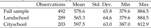
[image:19.595.160.405.318.364.2]The dependent variable is a difficulty-adjusted test score in reading. Table 1 re-ports the summary statistics of the score in our sample. We useOLSwith standard errors of the coefficients corrected for heteroscedasticity and common factors to students in the same school by clustering (cf. for a justification of this correction Froot, 1989, and Moulton, 1986).
Table 1
Summary statistics of reading performance.
Observations Mean Std. Dev. Min Max Full sample 492 578.6 65.8 379.6 884.5 Landschool 289 565.3 64.6 379.6 884.5 Cityschool 203 597.5 63.0 387.0 812.9
Obseravble input factors in educational production, such as class size and teacher qualification do not differ significantly between schools in rural and metropoli-tan areas. Hence, observed differences in student achievement must be due to differences in teacher motivation and school organization, which possibly result from diverse competitive settings.
4.3
Empirical Results
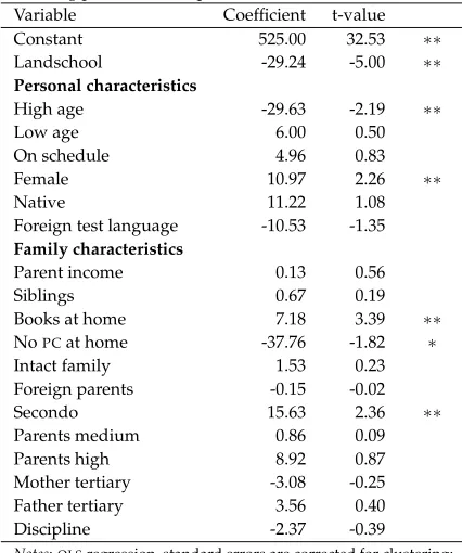
Table 2 displays the OLS regression results of estimating equation (13). Since we study matura schools across cantons, controlling for cantonal characteris-tics seems appropriate. It turns out, however, that including cantonal dummies yields no significant canton-specific factors in educational production. We hence exclude cantonal dummies from our estimation equation.
Table 2
Reading performance equation estimation. Variable Coefficient t-value Constant 525.00 32.53 ∗∗
Landschool -29.24 -5.00 ∗∗ Personal characteristics
High age -29.63 -2.19 ∗∗
Low age 6.00 0.50 On schedule 4.96 0.83 Female 10.97 2.26 ∗∗
Native 11.22 1.08 Foreign test language -10.53 -1.35
Family characteristics
Parent income 0.13 0.56 Siblings 0.67 0.19 Books at home 7.18 3.39 ∗∗
NoPCat home -37.76 -1.82 ∗
Intact family 1.53 0.23 Foreign parents -0.15 -0.02 Secondo 15.63 2.36 ∗∗
Parents medium 0.86 0.09 Parents high 8.92 0.87 Mother tertiary -3.08 -0.25 Father tertiary 3.56 0.40 Discipline -2.37 -0.39
Notes:OLSregression, standard errors are corrected for clustering;
number of observations: 492; number of clusters: 27;R2: 0.16;
∗∗denotes significance at the 5% level;
∗denotes significance at the 10% level.
points than students in schools which face direct competition. Personal charac-teristics significantly influencing test scores are a student’s high age and gender. High age means that a student had repeated a class due to unsatisfactory grades before the test was taken. It seems plausible that reading skills are somewhat autoregressive, such that this result is not surprising. We also find that female students perform better, which is a common finding acrossOECDcountries due to their higher maturity at that age.9
9PISAshows a pattern of gender differences that is fairly consistent across countries: In every
coun-try, on average, females reach higher levels of performance in reading literacy than males. The better performance of females in reading is not only universal but also large. On average, it is 32 points, and
Concerning family characteristics, the number of books at home, whether a stu-dent has access to aPCat home, and whether one of her parents is born abroad determines her performance significantly. The number of books can be inter-preted as an indicator of the parents’ attitude towards reading which influences their children’s reading capability. Whether a student has aPCat home also indi-cates her socioeconomic background which seems to be favorable if a student has the opportunity to use a computer. Interestingly, a student performs especially well if one of her parents was born abroad. One could argue that it is difficult for such children to attend matura school at all (because of a foreign first language, a different cultural background, etc.), so that they are particularly motivated to meet with success once they have this chance.
Besides the analysis of educational achievement (via test scores) as a function of regional characteristics, also educational attainment (via enrollment rates) could be analyzed in a similar setting. If school attendance is non-mandatory, students will choose to attend a certain school type only when their net-benefit from at-tending such a school is positive. As already laid out, attendance in matura school is voluntary, such that based on our model, one may expect that student participation in matura schools is higher in metropolitan areas than in rural ar-eas.
Figure 3 shows the location of matura schools in the canton of Z ¨urich as black dots. The ratio of students in matura schools and students in vocational school is indicated by the shading of the communities: The darker a community, the larger the fraction of matura students. The figure indeed suggests that children in communities farther away from matura schools tend not to attend matura school.
Figure 3
In the city of Z ¨urich, there are many schools close to each other, hence competing fiercely against each other and keeping their quality high, while schools in the rest of the canton face almost no competition with according performance of their students. Since more students participate in better schools, the metropolitan area around the city of Z ¨urich tends to show higher student attainment. Of course, in a more serious analysis of student attainment, one would also have to control for student characteristics, which would at least partly explain the high participation rates on the north-east bank of the lake (indicated by the white stripe in the south of the map).
5
Conclusion
We have modelled school organization and -finance in a framework where entry into the educational sector is free and where schools are heterogenous from a stu-dent’s perspective. The students’ success depends both on class size and spend-ing on schoolspend-ing resources. Abstractspend-ing from incentive issues within schools, we have analyzed the effect of competition between schools on student attainment. Higher government spending and fiercer competition – measured by the num-ber of schools in a district and lower transport cost – lead to an increase in the students’ educational achievement. This result confirms the findings in Hoxby (2000). Overall learning time in school is constant in the probability that students behave well if students are segregated by type. However, better behaving stu-dents profit more from schooling due to higher optimum resource spending for their classes.
6
Appendix
6.1
Proof to Result 1
Use the local student participation constraint (4) to see that
dsj
dmj
= Nejπ mlnπ
δ ,
dsj
dej
= Nπm
δ .
We thus have
dsj
dmj
=ejlnπ
dsj
dej.
Insert this into the first-order conditions (6) and (5) to find
m∗j =m∗ =− 1
lnπ,
where the first equality results from the symmetry of the schools. Note that by symmetrysj= NJ, and solve (5) foreto get
e∗j =e∗=max
0,m ∗g
ε −
δ
Jπm∗
where again the first equation results from the symmetry of the schools. Obvi-ously, the condition for an interior solution fore∗ismε∗g > δ
Jπm∗.
6.2
Proof to Result 2
Insertm∗ande∗from (7) and (8) respectively into (9) and solve forJ. Assuming an interior solution fore, we obtain (10).
6.3
Proof to Result 3
(a) Differentiatem∗with respect toπto find dmdπ∗ = 1
π(lnπ)2 >0. (b) Studying
time is given byπm. Differentiate with respect toπto get ddππm =0. (c) Substitute
m∗into (8), and differentiate with respect toπto get the result. (d) Substitutem∗
6.4
Proof to Result 4
(a)/(b) In order to find the optimum values ofm ande, given the number of schoolsJ, a benevolent planner solves the per-student problem
Π∗∗m,e: Wm∗∗,e= max
e,m∈R+
eπm− 1
mεe
.
The assumption that education takes place amounts to imposingπm > ε
m.
Ex-ploiting the first-order condition with respect tomyields
m: (m∗∗)2πm∗∗=− ε
lnπ ⇒m
∗∗<m∗,
where the inequality results from a comparison with (6). The first-order condi-tion with respect toeis
e: dW ∗∗
m,e
de >0.
(c) The efficient number of schools is determined by the social planner’s solution to the problem
Π∗∗
J : W∗∗J =Jmin∈R+
J f+Nδ
2J
1 2J Z 0 xdx .
She minimizes the sum of fixed costs plus the total transportation costs. The term in parenthesis represents the average transportation costs per person, where 21J is the farthest distance a student has to travel. Therefore, we have
J∗∗= 1
2
s
Nδ
f .
Thus, comparing with (10) yields
6.5
Proof to Result 5
The impact of increased government spending on welfare is
dΩ
dg =N dP∗
dg + Nδ
4(J∗)2
dJ∗
dg −N(1+λ)
=− N
εlnππ
− 1 lnπ +m
∗πm∗
f
4
dJ∗ dg
|{z} =0
−N(1+λ)
=− N
εlnππ
− 1
lnπ −N(1+λ).
6.6
Description of Variables
Table 3
Description of variables.
Variable Description
Read Weighted likelihood estimate in reading; difficulty adjusted test score
Landschool 1 if school location is in a city with up to 15’000 inhabitants; in our sample, this also means that there is only one school in that city.
Parent income Socio-economic index of parents’ occupational status as a proxy for income
Siblings Number of siblings
High age 1 if student is older than 204 months, 0 otherwise Low age 1 if student is younger than 180 months, 0 otherwise Books at home Number of books at home
On schedule 1 if student claims never to have arrived late in school during the last two school weeks, 0 otherwise
NoPCat home 1 if students has never accessed aPCat home, 0 otherwise Female 1 if student is female, 0 otherwise
Intact family 1 if pupil lives together with father and mother, 0 otherwise Native 1 if country of birth is Switzerland, 0 otherwise
Foreign Parents 1 if country of birth for both parents is not Switzerland, 0 otherwise
Secondo 1 if only one parent is born abroad, 0 otherwise Foreign test language 1 if native language is not testlanguage, 0 otherwise Parents medium 1 if parents’ highest level of education is lower secondary Parents high 1 if parents’ highest level of education is upper secondary Mother tertiary 1 if mother has tertiary education, 0 otherwise
Father tertiary 1 if father has tertiary education, 0 otherwise
No Discipline 1 if students feel disturbed by discipline problems at school
References
AMBLER, J. S. (1994): “Who Benefits from Educational Choice? Some Evidence from Europe,”Journal of Policy Analysis and Management, 13(3), 454–476.
CARNOY, M. (1997): “Is Privatization Through Education Vouchers Really the
Answer? A Comment on West,”World Bank Research Observer, 12(1), 105–116.
CAUCUTT, E. M. (2002): “Educational Vouchers When There are Peer Group Ef-fects – Size Matters,”International Economic Review, 43(1), 195–222.
DEFRAJA, G.,ANDP. LANDERAS(2004): “Could Do Better: The Effectiveness of
Incentives and Competition in Schools,”CEISTor Vergata Research Paper Series, 16(48).
ECONOMIDES, N. (1989): “Symmetric Equilibrium Existence and Optimality in Differentiated Product Markets,”Journal of Economic Theory, 47(1), 178–194.
EPPLE, D.,ANDR. E. ROMANO(1998): “Competition Between Private and Public
Schools, Vouchers, and Peer Group Effects,”American Economic Review, 88(1), 33–62.
FERTIG, M. (2003): “Who’s to Blame? The Determinants of German Students’ Achievement in thePISA2000 Study,”IZADiscussion Paper 739.
FIGLIO, D. N. (1999): “Functional Form and the Estimated Effects of School Re-sources,”Economics of Education Review, 18(2), 241–252.
FRIEDMAN, M. (1997): “Public Schools: Make Them Private,” Education Eco-nomics, 5(3), 341–344.
FROOT, K. A. (1989): “Consistent Covariance Matrix Estimation with Cross-Sectional Dependence and Heteroskedasticity in Financial Data,” Journal of Financial and Quantitative Analysis, 24(3), 333–355.
HOLMES, G. M., J. DESIMONE,ANDN. G. RUPP(2003): “Does School Choice
Increase School Quality?,”NBERWorking Paper 9683.
HOLMSTROM, B.,¨ ANDP. MILGROM(1991): “Multitask Principal-Agent
Analy-ses: Incentive Contracts, Asset Ownership, and Job Design,”Journal of Law, Economics and Organization, 7(Special Issue), 24–52.
HOXBY, C. M. (2000): “Does Competition Among Public Schools Benefit Stu-dents and Taxpayers?,”American Economic Review, 90(5), 1209–1238.
(2003): “School Choice and School Productivity: Could School Choice Be a Tide That Lifts All Boats?,” inThe Economics of School Choice, ed. by C. M. Hoxby, Chicago. The University of Chicago Press.
HOYT, W. H.,ANDK. LEE(1998): “Educational Vouchers, Welfare Effects, and
Voting,”Journal of Public Economics, 69(2), 211–228.
LADD, H. F. (2002): “School Vouchers: A Critical View,”Journal of Economic Per-spectives, 16(4), 3–24.
LAZEAR, E. P. (2001): “Educational Production,”Quarterly Journal of Economics,
66(3), 777–803.
LEVIN, H. M. (2002): “A Comprehensive Framework For Evaluating Educa-tional Vouchers,”Educational Evaluation and Policy Analysis, 24(3), 159–174.
MCMILLAN, R. (2004): “Competition, Incentives, and Public School Productiv-ity,”Journal of Public Economics, 88(9-10), 1871–1892.
MOULTON, B. R. (1986): “Random Group Effects and the Precision of Regression Estimates,”Journal of Econometrics, 32(2), 385–397.
NEAL, D. (2002): “How Vouchers Could Change the Market for Education,” Jour-nal of Economic Perspectives, 16(4), 25–44.
NECHYBA, T. J. (1996): “Public School Finance in a General Equilibrium Tiebout
World: Equalization Programs, Peer Effects and Private School Vouchers,” NBERWorking Paper 5642.
(1999): “School Finance Induced Migration and Stratification Patterns: The Impact of Private School Vouchers,”Journal of Public Economic Theory, 1(1), 5–50.
OECD (2001): Knowledge and Skills For Life. Organization for Economic Co-Operation and Development, Paris.
PRITCHETT, L.,ANDD. FILMER(1998): “What Education Production Functions
Really Show: A Positive Theory of Education Expenditures,”Economics of Ed-ucation Review, 18(2), 223–239.
SALOP, S. (1979): “Monopolistic Competition with Outside Goods,”Bell Journal of Economics, 10(1), 141–156.
SIDOS (2004): “PISA 2000 – Program for International Student Assessment,”
http://www.sidos.ch.
TIROLE, J. (1988): The Theory of Industrial Organization.MITPress, Cambridge, MA.
WEST, E. G. (1997): “Education Vouchers in Principle and Practice: A Survey,”
World Bank Research Observer, 12(1), 83–103.
W ¨OSSMANN, L. (2004): “How Equal are Educational Opportunities? Family
Background and Student Achievement in Europe and the United States,”IZA