Munich Personal RePEc Archive
Application of machine learning to
short-term equity return prediction
Yan, Robert and Nuttall, John and Ling, Charles
3 April 2006
Online at
https://mpra.ub.uni-muenchen.de/2536/
APPLICATION OF MACHINE LEARNING TO
SHORT-TERM EQUITY RETURN PREDICTION
Robert J. Yan
University of Western Ontario
John Nuttall
University of Western Ontario
Charles X. Ling University of Western Ontario
April 3, 2006
ABSTRACT
1. INTRODUCTION
In the past studies have discovered a considerable number of 'anomalies' that suggest
that stock returns are predictable by using information available at the time the stock is
bought. Moreover the many people in the investment industry that manage active equity
portfolios must believe that stock returns are to some extent predictable. Yet there are
many others, particularly in the academic community, who believe that the evidence of
predictability is completely or largely spurious and/or irrelevant, using arguments such as
The profit resulting from any practical method of using the supposed
predictability will disappear after taking account of trading and information
costs;
Results supporting the existence of predictability were obtained after simulating
past returns based on a large set of possible anomalies and reporting only those
few that by chance showed high returns, i.e. they are due to snooping;
Even if precautions to minimize snooping had been taken, market conditions
might change in the future so that the anomaly disappears.
All these questions merit serious consideration, and we must accept that there will
never be definitive answers one way or the other. However, many of the doubters about
the existence of predictability seem to exhibit an almost religious fervor [Lo and
Mackinlay 1999] rather than approaching the problem as a dispassionate scientist should.
They concentrate exclusively on objections to the studies that suggest predictability,
without making any attempt to determine whether the methods of the studies might have
It is from this point of view that we examine the work of Cooper [Cooper 1999], in
particular Section 3 devoted to a real-time simulation of filter strategies to predict
one-week stock returns based on price and volume data for the previous two one-weeks. We
observe that Cooper's implicit method of return prediction may be regarded as a primitive
application of the principles of Machine Learning (ML see for instance [Hastie,
Tibshirani, and Friedman 2003 Mitchell 1997]). We propose and apply to this case a
new variant of a ML method (called the PKR method) designed specially for the problem
at hand. Our work strongly suggests that the return predictability of Cooper's method
could have been increased by the use of ML. It is of interest to note that what we have
done could have been done years ago by someone who had the requisite contemporary
knowledge of ML and financial economics.
We note that we and other authors are interested only in measuring the accuracy of
significantly high or low return predictions, since the accurate prediction of roughly
average returns does not appear to have much economic value. That is what we take the
term 'return predictability' to mean throughout this report.
To obtain a measure of the value of his return predictions Cooper formed weekly a
portfolio of stocks chosen using those predictions. Following Cooper and the precepts of
ML, we do our best to mitigate the dangers of snooping. Over a period of many weeks the
measure of predictability is given by the performance of the portfolio, such as average
return, volatility, etc. Since our aim is to compare the return predictability of Cooper's
method with our ML method, we have used a different, simpler way of forming
portfolios, because Cooper's portfolio construction method is difficult to apply to our
due entirely to differences between the two return prediction methods. We show that
portfolio returns over a long period would have been consistently higher for the new
method as compared to Cooper's (implicit) method. Implications for the Efficient Market
Hypothesis [Fama 1970] are discussed.
Section 2 describes the general framework of machine learning that we use to develop
a stock return prediction system, and its application in the style of Cooper and in the new
PKR form. Section 3 explains the common portfolio construction scheme used to
evaluate both methods of return prediction, and compares results for the two cases.
Section 4 concludes with a discussion.
2. MACHINE LEARNING AND RETURN PREDICTION
2.1. BASIC STRUCTURE
We assume that trading days (when the market is open) are divided into 'weeks' of
five days labelled by the index t. Our task is to find the predicted return RP(j,t) of each stock j in the set (universe) of stocks that we choose for week t, given only information available at the start of the week. The process that we (or any investment manager)
use may be formally written as
t
Φ
( , ) ( , t),
RP j t =GP j Φ (1)
where GP describes the procedure, mathematical or otherwise, that transforms the data
Cooper [Cooper 1999], and many other writers on anomalies, implicitly assume that
the information used to construct RP(j,t) is a function of a small number M of predictors
P(i,j,t), i=1,...,M, so that we write
( , ) ( ( , ), ),
RP j t =G P j t t (2)
where P(j,t)is a vector with components P(i,j,t), i=1,...,M.
We stress that the above framework assumes that the predicted return of stock j
depends only on the predictors associated with that stock, and that the prediction function
for stock j is independent of j apart from the dependence on P(j,t). In principle both these assumptions could be relaxed.
There remain two key decisions to be made.
What choice to make for the predictors?
How to find the function G(X,t)?
2.2. PREDICTORS
We follow Cooper [Cooper 1999] in the choice of predictors and define them as:
Predictor 1 P(1,j,t) = the return of stock j for the week t-1. Note that we do not include a lag day.
Predictor 2 P(2,j,t) = the return of stock j for the week t-2
Predictor 3 P(3,j,t) = volume value ratio defined as 1 1 2
V V V V
2
−
+ , where V1, V2 are
transformation of Cooper's volume value ratio that leads to a more symmetric
distribution of values.
We also provide results for the six subsets of these predictors, i.e. one at a time and
two at a time.
2.3. PREDICTION FUNCTION
The prediction function G(X,t) at any given time t is found by a process known as
'learning'. The information used by the learning process is contained in samples
, where R(j,k) is the actual return for stock j in week k. When
determining G(X,t), the learning process may use information in any samples such that both the predictor vector P(j,k) and the return R(j,k) are known at time t, so that we require k < t. We define SPRED(t) to be the set of samples chosen for use in the learning process at time t.
( , ) { ( , ), ( , )}
S j k = P j k R j k
In essence the idea is to find the acceptable function G(X,t) that comes closest to satisfying the relation
( ( , ), )) ( , )
G P j k t =R j k (3)
for all samples S(j, k) that we decide to use in the learning process at time t, i.e. the set
SPRED(t).
A standard approach is to choose a family of possible forms for the prediction
function, GFAM(X,t,W), where W ={ ( ),W i i=1,L,MW} is a vector of MW parameters
W(i) that specify the function. The problem of finding G(X,t) is reduced to the question of finding the particular parameter vector W so that GFAM(X,t,W) is the acceptable function of X that is nearest to satisfying
GFAM P j k t W( ( , ), , )=R j k( , ), (4)
for all j, k with S(j, k) in SPRED(t).
This problem, a key part of ML, is the subject of the branch of mathematics known as
Approximation Theory [Cheney 2000].
2.4. COOPER'S METHOD
To find the return prediction function for week t Cooper first, for each predictor, divides into deciles the historical distribution of predictor values for a previous period
that includes all the stocks and weeks corresponding to the samples in SPRED(t). Using the decile boundary values, the three-dimensional space of predictor values is partitioned
into 1000 cells, with each cell corresponding to a choice of three decile numbers. Let us
call the cells CL(i), i = 1, ... ,1000. The treatment is analogous for cases with one or two predictors.
We define RCL(t,i) to be the average of the one-week returns of all stocks in cell
CL(i) in the weeks in the above period. Effectively, although he does not state it explicitly, Cooper assumes that the predicted return of stock j for week t is
( , ) ( , )
where ia=LAB P j t( ( , )), i.e. label of the cell that contains the predictor vector P(j,t).
Note that this means that Cooper's version of the prediction function G(X,t) is piecewise constant in the 3-dimensional predictor space with coordinate X. Filter methods used by other authors may be interpreted in the same way as we have done for Cooper's.
This result may be derived in the general framework described above. Thus we
choose the family of prediction functions to be
1000
1
( , ) ( , , ) ( ) ( , )
i
G X t GFAM X t W W i STP X i
=
= =
∑
× , (6)where the step function STP is defined as
1: if ( )
( , ) ,
0 : otherwise
i LAB X STP X i = ⎨⎧ =
⎩ (7)
If we choose
( ) ( , )
W i =RCL t i , i=1, ... , 1000
we obtain a result equivalent to (4). It may be shown that this choice of W minimizes the mean square error between the two sides of (4).
2.5. PKR METHOD
When designing a ML method we must consider the character of the data contained
in the samples SPRED(t), and also how we intend to use the prediction function G(X,t). We note the following points.
The sample set that Cooper used for learning contained 300 stocks for say 50
In contrast to Cooper we would like to extend the data set on a weekly basis so
that the prediction takes account of the latest available data. The method for
computing G(X,t) should be designed so that the total time for computations is acceptably low;
Compared to most applications of ML the data is noisy. The distribution of the
values of R(j,k) corresponding to a neighbourhood of predictor space is wide;
The density of samples in predictor space is high for moderate values of the
predictors but low for extreme values. Note that the density of samples can be
changed by transforming the predictor variables;
We expect that the more extreme values of G(X,t) that we desire will occur where the sample density is lower.
Apart from the constraint on computing time, the kernel regression method [Hardle
1990 Wand 1994] is a good candidate for the process to use to find G(X,t). In that method the prediction function is given by
,
1
( , ) ( , ( , )) ( , ),
( , ) ( ) and ( , ) ( ),
j k
GKR X t K X P j k R j k WKR
S j k SPRED t P j k NBD X
= ×
∈ ∈
∑
(8)
where the kernel K X Y( , )is often chosen as
2
(X Y)
e⎡⎣−μ − ⎤⎦, and the weight WKR is
,
( , ), ( , ) ( ) and ( , ) ( ),
j k
WKR=
∑
K X Y S j k ∈SPRED t P j k ∈NBD X (9)The effect of the kernel regression method is to approximate the return at a point Xin predictor space by an average of the returns for nearby samples, weighted to emphasize
the nearest samples. The averaging tends to reduce the noise in the sample returns. This
method produces a result that is smooth in X, in contrast to the cell method used by Cooper. In addition the kernel regression method will lead to return predictions in low
density regions of predictor space that are not dominated by sample returns in high
density regions, in contrast to global methods such as neural networks.
The drawback to the kernel regression method in the present application is the time
taken to perform the computations if we make predictions every week using the latest
data. To reduce computing time by a large factor without losing much accuracy, we have
designed a modified kernel regression method that we call the Prototype Kernel
Regression method (PKR). The steps in the PKR method are
Choice of prototype points
We choose a set of points called prototypes Q(i), i=1,...,MP, distributed through predictor space, where MP is much smaller than the number of samples in
SPRED(t). The prototypes are fixed for many weeks. In the current application we chose to place the prototype points on a regular rectangular grid;
Estimate return at the prototype points
We use the standard kernel regression method to estimate the predicted return at
the prototype points. For the neighbourhoods we chose the cells in the grid that
have the prototype point as a corner. The calculations involved change from
and we save a lot of time by using a recursive operation to take advantage of
this structure;
Estimate the return at the sample points each week
To find the predicted return at each sample point for a given week (300 points in
the case of Cooper) we apply the kernel regression method where we take the
values at the prototype points as input samples. The neighbourhood contains the
corners of the cell that includes the sample predictor vector.
3.
PORTFOLIO CONSTRUCTION AND RESULTS
In order to evaluate the accuracy of the stock returns predicted by his method, Cooper
[Cooper 1999] constructs portfolios of groups of stocks, with a group consisting of an
equally weighted combination of all the stocks in a given cell. Since the choice of cell
boundaries is arbitrary and not likely to be of real significance in predicting returns,
Cooper's approach is open to question. Moreover, our PKR method does not involve
cells, so that it is not clear how to apply Cooper's method.
Consequently we have used a simple alternative portfolio formation scheme to
evaluate the return predictability of both methods. Each week we form a neutral portfolio
consisting of N stocks long and N stocks short. The long (short) stocks are those with highest (lowest) predicted return. Each stock has equal weight (except when there are
several stocks tied for last place, when all those stocks are chosen with equal reduced
weight). The returns of these portfolios are what we study.
The study covers the period 1963 - 2004. The stock universe is revised monthly. It
consists of the 300 NYSE and AMEX stocks from the CRSP database that have the
largest market capitalization. In all 504 different stocks were chosen.
3.2. PROCEDURE
The universe that applies to any given week of five trading days is the latest of those
chosen above with a date earlier than the first day of the week. In a given week we omit
any stock that has missing volume information for any of the previous ten days.
For the set of samples SPRED(t) used for learning in week t we choose all samples relating to weeks prior to week t. Thus the set of samples continually increases in size, but always includes the most recent available samples. We choose stocks as described
above and calculate neutral portfolio weekly return as a percent of the amount invested
long each week.
3.3. RESULTS
We generate results for several cases specified by the following parameters.
Choice of return prediction method:
CF - our version of Cooper's filter method;
PKR - our method of machine learning;
Choice of number of stocks:
The number of stocks N in long and short portfolios. Choose N = 5,10,...,50;
Choice of predictors:
For each combination of the above choices we calculate portfolio statistics (average
weekly return before any costs and standard deviation) for the periods 1964 - 1977, 1978
- 1993, 1994 - 2004. We chose the middle period 1978 - 1993 because that was the one
Cooper used for his tests.
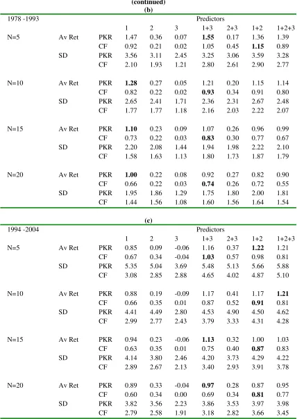
[image:14.612.96.516.390.679.2]In Table 1 we provide results for the values N = 5, 10, 15, 20, which are of most interest. Some features of these results are as follows.
Table 1. Percentage weekly returns of portfolios formed using return predictions by the PKR and CF methods.
Neutral portfolios are formed with N equally weighted stocks long (short) chosen on the basis of the highest (lowest) predicted returns. For each of the three indicated periods this is done using 7 combinations of the three predictors. The table shows the average and standard deviation of the weekly portfolio percentage returns for the two prediction methods PKR and CF.
(a)
1964 -1977 Predictors
1 2 3 1+3 2+3 1+2 1+2+3
N=5 Av Ret PKR 1.32 0.51 0.15 1.19 0.54 1.57 1.21
CF 0.94 0.36 0.15 0.84 0.48 1.30 0.73
SD PKR 3.04 2.81 2.36 2.88 2.87 3.18 3.17
CF 1.73 1.76 1.11 2.32 2.55 2.64 2.92
N=10 Av Ret PKR 1.22 0.54 0.13 1.17 0.50 1.30 1.09
CF 0.89 0.37 0.15 0.81 0.42 1.14 0.63
SD PKR 2.20 2.06 1.71 2.08 2.11 2.31 2.16
CF 1.52 1.56 1.10 1.73 1.96 2.10 2.09
N=15 Av Ret PKR 1.09 0.48 0.12 0.99 0.52 1.17 1.01
CF 0.83 0.38 0.15 0.77 0.40 1.03 0.61
SD PKR 1.79 1.84 1.41 1.75 1.82 1.96 1.85
CF 1.39 1.43 1.08 1.49 1.71 1.76 1.70
N=20 Av Ret PKR 1.00 0.47 0.08 0.92 0.45 1.07 0.98
CF 0.78 0.39 0.15 0.73 0.40 0.96 0.59
SD PKR 1.59 1.64 1.23 1.55 1.67 1.73 1.63
Table 1 (continued)
(b)
1978 -1993 Predictors
1 2 3 1+3 2+3 1+2 1+2+3
N=5 Av Ret PKR 1.47 0.36 0.07 1.55 0.17 1.36 1.39
CF 0.92 0.21 0.02 1.05 0.45 1.15 0.89
SD PKR 3.56 3.11 2.45 3.25 3.06 3.59 3.28
CF 2.10 1.93 1.21 2.80 2.61 2.90 2.77
N=10 Av Ret PKR 1.28 0.27 0.05 1.21 0.20 1.15 1.14
CF 0.82 0.22 0.02 0.93 0.34 0.91 0.80
SD PKR 2.65 2.41 1.71 2.36 2.31 2.67 2.48
CF 1.77 1.77 1.18 2.16 2.03 2.22 2.07
N=15 Av Ret PKR 1.10 0.23 0.09 1.07 0.26 0.96 0.99
CF 0.73 0.22 0.03 0.83 0.30 0.77 0.67
SD PKR 2.20 2.08 1.44 1.94 1.98 2.22 2.10
CF 1.58 1.63 1.13 1.80 1.73 1.87 1.79
N=20 Av Ret PKR 1.00 0.22 0.08 0.92 0.27 0.82 0.90
CF 0.66 0.22 0.03 0.74 0.26 0.72 0.55
SD PKR 1.95 1.86 1.29 1.75 1.80 2.00 1.81
CF 1.44 1.56 1.08 1.60 1.56 1.64 1.54
(c)
1994 -2004 Predictors
1 2 3 1+3 2+3 1+2 1+2+3
N=5 Av Ret PKR 0.85 0.09 -0.06 1.16 0.37 1.22 1.21
CF 0.67 0.34 -0.04 1.03 0.57 0.98 0.81
SD PKR 5.35 5.04 3.69 5.48 5.13 5.66 5.88
CF 3.08 2.85 2.88 4.65 4.02 4.87 5.10
N=10 Av Ret PKR 0.88 0.19 -0.09 1.17 0.41 1.17 1.21
CF 0.66 0.35 0.01 0.87 0.52 0.91 0.81
SD PKR 4.41 4.49 2.80 4.53 4.90 4.50 4.62
CF 2.99 2.77 2.43 3.79 3.33 4.31 4.28
N=15 Av Ret PKR 0.94 0.23 -0.06 1.13 0.32 1.00 1.03
CF 0.63 0.35 0.01 0.75 0.40 0.87 0.83
SD PKR 4.14 3.80 2.46 4.20 3.73 4.29 4.22
CF 2.89 2.67 2.13 3.40 2.93 3.91 3.78
N=20 Av Ret PKR 0.89 0.33 -0.04 0.97 0.28 0.87 0.95
CF 0.60 0.34 0.00 0.69 0.34 0.81 0.77
SD PKR 3.82 3.56 2.23 3.86 3.53 3.97 3.98
1. On their own Predictors 2 and 3, the return for the week two weeks before the
holding week and the volume ratio, have little power for all periods and numbers of
stocks whether we use the PKR or the CF prediction method. Not surprisingly the same
goes for the combination of predictors 2 and 3. In the subsequent discussion we shall
concentrate on the four remaining combinations of predictors that are used to construct
portfolios, i.e. Combinations 1, 1+2, 1+3, 1+2+3.
2. The average weekly returns for all periods, numbers of stocks, and four predictor
combinations, and methods, 96 in total, are positive.
3. In all cases out of 48 the average return for the PKR method is greater than that for
the CF method. The average margin of one over the other is 37.0%.
4. The average margin of the ratio avRet/sd for the 48 cases is 13.0% in favor of the
PKR method, but that ratio has little meaning until costs are included.
5. The choice of the predictor combinations that leads to the highest average return
for given period and N varies over the 12 cases, as shown in Table 2. Note that the high return combinations change from period to period. Also note that, apart from the period
64 - 77, the combination with the highest return for a given period and N changes from PKR to CF, but often other combinations have a return that is little different from the
Table 2. Distribution of highest portfolio returns by predictor combination.
For the 12 cases corresponding to 3 periods and 4 values of N (number of stocks) listed in Table 1, the table shows how many times a particular combination of predictors has highest average weekly return.
Predictor combination 1 2 3 1+3 2+3 1+2 1+2+3
No. of cases PKR 3 0 0 3 0 5 1
CF 0 0 0 4 0 8 0
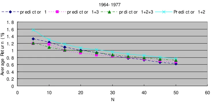
6. Generally, in the PKR case for a given period and choice of predictor combination,
the average return increases steadily as N decreases from 50. Four cases are exceptional in Period 94 - 04, where with Combinations 1, 1+3 and 1+2+3 the return decreases for N
= 5, and similarly Combination 1 for N = 10. See Figure 1 where results for the three high return combinations are plotted.
Figure 1. Weekly average return plotted against N (number of stocks) and period for the four most
important predictor combinations.
1964- 1977
0 0. 2 0. 4 0. 6 0. 8 1 1. 2 1. 4 1. 6 1. 8
0 10 20 30 40 50 60
N
A
v
er
age R
e
t
ur
n (
%
)
[image:17.612.117.482.398.575.2]1978- 1993 0 0. 2 0. 4 0. 6 0. 8 1 1. 2 1. 4 1. 6 1. 8
0 10 20 30 40 50 6
N A v er age R et ur n ( 5) 0
pr edi ct or 1 pr edi ct or 1+3 pr di ct or 1+2+3 pr edi ct or 1+2
1994- 2004 0 0. 2 0. 4 0. 6 0. 8 1 1. 2 1. 4 1. 6 1. 8
0 10 20 30 40 50 6
N A v er age R et ur n ( % ) 0
pr edi ct or 1 pr edi ct or 1+3 pr di ct or 1+2+3 pr edi ct or 1+2
4.
DISCUSSION
4.1. PROFITABILITY AND COSTS
Our results provide strong support the view that four combinations of the three
predictors have pre-cost predictive power in all three periods studied, whether we use the
Cooper method of prediction or our new PKR method. Without exception the PKR
method produces higher average pre-cost returns, on average 37% higher. This number
before making the comparison. There will be a range of cost levels where the PKR
method would make a profit but the CF method a loss.
The fact that, for a given period and combination of predictors, the PKR average
return generally increases steadily as the number of stocks N decreases, reinforces the view that the PKR method produces meaningful predictability. If our ranking of predicted
stock returns was accurate then this behavior would be observed. The two exceptions to
the general trend occur at low N in the period 1994 - 2004 and may be attributable to the higher noise level in that period and for lower N.
4.2. EFFICIENT MARKET HYPOTHESIS
The Efficient Market Hypothesis (EMH) comes in several flavors. In terms of
practical applicability Malkiel [Malkiel 2003] expresses a widespread view that
"Evidence is overwhelming that no anomalous behavior of stock prices creates a
portfolio trading opportunity that enables investors to earn extraordinary risk adjusted
returns."
Supporters of this view would argue that Cooper's work does not contradict this form
of the EMH because the costs would wipe out any economic profit indicated by his
results.
Without reliable information as to what the costs would have been it is impossible
come to a definitive conclusion. However, it is reasonable to suppose that the costs for
Cooper's method and our PKR method would have been similar. We have provided
of Cooper's method. This means that the proponents of the EMH now have to
demonstrate the existence of a higher level of realistic costs than was required to show
that Cooper's results were inconsistent with the EMH. The cost hurdle for EMH
advocates has been raised. It is quite likely that the same applies to other anomalies
previously studied, in that improved methods of Machine Learning might well improve
their pre-cost returns.
4.3. CHOICE OF PREDICTOR COMBINATIONS
Cooper discusses the case when an investor forms weekly portfolios during the period
1978 - 1993 using information available at the time that may go back as far as 1963.
Cooper's portfolio construction method differs from ours, but roughly, in our context, the
procedure would be to use at any time a subset of the four useful predictor combinations
to form the current portfolio. That subset could be chosen on the basis of what worked
best in the past 15 years. Our results show that the choice would change from time to
time. In this report we have not attempted to study how best to make this choice, but the
general problem is of great importance to investment managers.
Acknowledgement
We appreciate the access to the CRSP database provided by the University of
References
1. Cheney, E. W. 2000. Introduction to Approximation Theory.: Amer Mathematical Society.
2. Cooper, M. 1999. Filter rules based on price and volume in individual security overreaction. Review of Financial Studies 12, no. 4:901-935.
3. Fama, E. 1970. Efficient Capital Markets: A Review of Theory and Empirical Work. Journal of Finance 25, no. 2:383-417.
4. Hardle, W. 1990. Applied Nonparametric Regression.: Cambridge Univ. Press.
5. Hastie, T., R. Tibshirani, and J. H. Friedman. 2003. The Elements of Statistical Learning.: Springer.
6. Lo, A. W. and A. C. Mackinlay. 1999. A Non_Random Walk Down Wall Street.: Princeton University Press.
7. Malkiel, B. G. 2003. The efficient market hypothesis and its critics. Journal of Economic Perspectives 17, no. 1:59-82.
8. Mitchell, T. 1997. Machine Learning.: McGraw Hill.