An Econometric Model of Tourism Demand in France

An Econometric Model of Tourism

Demand in France

Botti, Laurent and Peypoch, Nicolas and Randriamboarison,

Rado and Solonandrasana, Bernardin

University of Perpignan, University of Perpignan, University of

Perpignan, University of Perpignan

7 July 2006

AN ECONOMETRIC MODEL OF TOURISM DEMAND

IN FRANCE

Laurent Botti1

University of Perpignan

Nicolas Peypoch

University of Perpignan

Rado Randriamboarison

University of Perpignan

Bernardin Solonandrasana

University of Perpignan

This case study gives an overview of the tourism demand in France by using an econometric model. The study covers the period between 1975 and 2003. Five developed countries have been selected, and the choice of the countries is based upon the fact that continuous data on all relevant variables are available only for those countries. The results show a positive relationship between tourist expenditures and generating country GDP, and a negative relation between tourist expenditures and relative prices.

Keywords: tourism demand, tourist expenditures, national income, relative prices.

INTRODUCTION

Many authors have written about the important role played by tourism industry in the economy in general and in development in particular. During the second half of the twentieth century, tourism has become one of the main economic activities that have recorded the most important growth. As a matter of fact, in the 30-year period since the 1950s toward the end of the 1980s, total international tourist flows have grown by a factor of six, to approximately 400 millions (Chu, 1998). Such a rapid expansion of tourism is linked to two main reasons: (i) first the increase of available income of wage earners in the majority of developed countries and the decrease of the working-time, thereby an increase of the

spare-time. (ii) Second, the decrease of the transport charges between two destinations taking into account the considerable development of means of transport.

In 2004, France remained to be the first international destination in terms of number of arrivals. With a number of tourists reaching up to 75,1 millions, France is far ahead compared to countries such as Spain (53,6 millions), United States of America (46,1 millions), or China (41,8 millions). The account of the balance of payments shows a positive sign procuring to France 10,7 billions euros of receipts, representing therefore an increase of 7,5% compared to the year 2003. In that case, the sector of tourism constitutes a major issue for France. Forecasting tourism demand appears to be more than necessary for the well-being of the French economy.

Several techniques in forecasting tourism demand are currently available. Witt and Witt (1995) and Li, Song and Witt (2005) provide very interesting surveys in this field. Randriamboarison (2001) has recorded 163 empirical studies on tourism demand through use of quantitative approaches for the period starting from 1963 to 2003. The number of arrivals, the tourist expenditures, and the tourist receipts are utilised as dependant variables. As for explicative variables, we have the national income, the exchange rate, the total number of population, the price and one or more dummy variables showing a specific event in the hosting country. Econometric problem also causes the authors to include the trend and an others variables to the explicative variables. In most of the cases, data are annual. Lim (1997:837) point out that to circumvent the problem related to the unavailability of long time series of annual data, some studies used monthly, quarterly, cross-section, and pooled annual and cross-section data, or a combination of these.

models is very possible. Likewise, we can talk about problem of co-integration. In order to address the problem, Smeral, Witt and Witt (1992) and Akis (1998) are using a model with two explicative variables, such as the national income and relative prices. The results are satisfying according to them.

In spite of such results, tourism industry is a field within only a few numbers of French economists are working. The aims of this study are to bring more light on the evolution of the tourism demand in France. It offers to examine the relationship between demand, national income and relative prices. The approach used by Smeral, Witt and Witt (1992) and Akis (1998) will be adopted but this time by also applying the test of stationarity in order to ensure that there is no false linear relation in the model. The five countries taken in the study are Germany, the United States of America (USA), Spain, Italy and the United Kingdom (UK). The annual data used are covering the period between 1975 and 2003.

MODELLING TOURISM DEMAND IN FRANCE

France is seen as the leading country in the area of international tourism and this can be explained by the remarkable tourism richness of the country: its 22 tourism regions receiving in 2003, 75,1 millions arrivals, that is to say approximately 10% of world total of tourists. In 1998, during the year of the World Cup of football, 70 millions arrivals were registered. According to Peyroutet (1998), the visitors are mainly attracted first by touring the cities (31%), then the coast, the mountains and the countryside. The most commonly chosen regions are Provence-Alpes-Côte d’Azur (103,7 millions of overnight stay), Rhône-Alpes (92,1 millions of overnight stay) and Languedoc-Roussillon (76,8 millions of overnight stay). France has, presently, about 13 000 edifices classified as patrimony. All of them are considered as being the tourism offer of France. Such a patrimony consists of historic and prehistoric sites, religious edifices, castles, manors, and civil buildings.

Table 1. The 5 most visited monuments

Monuments Visitors

Louvre 6 600 000

Table 1 shows the most visited monuments in France. Besides, the country has 7 500 protected sites and 140 natural reserves.

Concerning the accommodation: in 2004, France offers to its tourists a range of 27 641 registered hotels from 1 to 4 luxury stars unequally allotted in its 22 regions. Furthermore, there are 8 059 registered camping areas from 1 to 4 stars; 813 registered holiday villages, 217 inns, and 41 957 rural as well as communal lodges and 22 053 guesthouses. The supply of tourist stopping points is summarized in table 2.

Table 2. Offer of tourist stopping point (in 2004)

Registered hotels 1 230 800 Classified camping 2 803 900 Holiday Villages 607 000

Inn 18 000

Lodges and guesthouses 266 000

It is rather difficult to express the number of jobs created, however official data show that the sector of tourism employ independent workers or wage earners. The totals of the assets in tourism are 975 300 on direct employment. Important numbers small family businesses also exist. In France, an increase of 13% of the number of workers in tourism between 1990 and 2004 is recorded. In terms of income, as previously mentioned, tourism has generated a total of 40,8 billions euros for the year 2004 in France. The account balance is regularly positive since 1963 (9,8 billions euro in 2004).

Model and data

In elaborating an econometric model, the choice of the function is always the first step. The general international tourism demand model typically estimated is:

DTij = f(Yj ,TCij ,RPij ,ERij ,QFi )

where:

DTij = demand for international travel services by origin j for destination i;

Yj = national income of origin j;

TCij =transportation cost between destination i and origin j;

RPij = relative prices, the ratio of prices in destination i to prices in origin j;

ERij = exchange rate, measured as units of destination i’s currency per unit of

origin j’s currency;

QFi = qualitative factor in destination country i.

paramount in the determination of a specific functional form for purposes of estimation and testing. Two types of models are then used towards the determination of such specificity: the linear model and the log-linear model or double-logarithmic. Quayson and Var (1982) used the transformation of Box-Cox to compare the linear and log-linear models. They came to the conclusion that the log-linear specification is more robust. In the same way, Oum (1989, p.165) have also stated some advantages of the log-linear model: (a) the coefficients themselves are the respective elasticities of the demand; (b) the log-linear function is capable of modelling non-linear effects; (c) it resembles the demand function obtainable from a Cobb-Douglas utility (production) function; and (d) it permits the random errors in the equation to be normally distributed. As for us, we are going to adopt the log-linear model, the model that is close to the economic hypothesis on demand: derivability, convexity of preferences and desirability.

The second step of the elaboration of the model is the choice of the variables. By referring to the traditional theory, it is said that consumer’s demand function is the function associated to a price-vector P and to an income R, the optimal choice of the consumer (Guerrien 1989:49). In that case, demand is linked to the price and income. In the case of international trade, the evolution of the importation demand is linked not only to income of the country transacting the importation, but also to the relative price which is the international price divided by domestic price. As far as tourism demand is concerned, such a demand depends on the income of the generating country. Demand depends as well as on the relative prices between the origin country and the destination country. After considering such theory-based and practical explanations, we can therefore draw our function on tourism demand in France as follows:

i ij j

ij LogGDP LogRP

LogD = β₁ +β₂ + β₃ +ε

where:

ij

D = Tourist expenditures from country j to country i;

j

GDP = Income from the origin country j; ij

RP = Relative prices; i

ε

Concerning the explicative variables, we have the income of tourist-generating country. In this study such a variable is represented by the GDP, in the constant price. The use of the available income appears to be more relevant but data on such a variable are not available. GDP of the EU countries were taken from the Eurostat while the ones for the USA, UK come from the “Economie Européenne”. The problem is how to measure relative prices. Transforming data was an inevitable necessity in order to determine relative prices. The formula used to calculate the relative prices of all countries taken in the sample is:

⎟ ⎠ ⎞ ⎜ ⎝ ⎛ = ij j i ij ER IPC IPC RP * where:

IPCi = consumer price index of the destination country;

IPCj = consumer price index of the tourist generating country;

ERij = exchange rate.

For example, the relative price between France and Germany is given by the consumer price index in France divided by the consumer price index in Germany, multiplied by the exchange rate between French Francs and Deutsch Mark. The series of those variables were excerpted from World Tables and the variable exchange rate of the “Economie Européenne”.

As a first step, the order of integration of our series is determined through the application of some stationarity tests. Those series will be corrected by having recourse to differentiation with order of integration. The equation is estimated by ordinary least squares (OLS). That leads us in a second step to the following conclusion: the model is deemed to be satisfying if it shows the real sign of the coefficient. In our case, the sign of the coefficient borne by income should be positive. An increase of income will lead to the increase of tourist expenditures. The real sign of the coefficient borne by relative prices is negative, the demand being a decreasing function of the price. In other words, we have an elasticity price of the demand negative. There will be a decrease in expenditures following an increase of the price. Besides, the coefficients have to be significant different of zero following the value of the t-Student. The Durbin-Watson (DW) is also used in decision-making. The DW indicates the absence (or likely absence) of autocorrelation. The F statistic has to be a high value. A low value of the F statistic suggests that the equation is not, in general, significant. The coefficient R2 should be close to 1.

Empirical results

used to test our variables for a unit root in its level, and then in the first difference form. Table 3 presents testing results for tourist expenditures variable, table 4 for the GDP variable and table 5 for the relative prices.

Table 3. ADF tests on expenditures

Countries Tourist expenditures

Level form First difference form With C & trend None With C & trend None

Germany -1.90 2.08 -2.05 -2.65 * *

USA -1.82 1.22 -4.33 * -6.65 * *

UK -1.87 2.49 -3.89 * -2.83 * *

Italy -2.69 2.12 -2.72 -2.14 *

Spain -2.63 0.85 -3.74 * -3.81 * *

**, statistical significant at the 1 percent level *, statistical significant at the 5 and 10 percents level

Table 4. ADF tests on GDP

Countries GDP

Level form First Difference Form With C & trend None With C & trend None

Germany -2.16 -0.57 -2.92 -3.07 **

USA -1.97 -1.71 -2.57 -2.68 **

UK -2.09 0.29 -3.07 -3.06 **

Italy -4.91 * -1.58 -6.22 ** - 5.17 ** Spain -2.45 1.76 -4.29 ** -4.49 **

**, statistical significant at the 1 percent level *, statistical significant at the 5 and 10 percent level

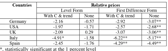
Table 5. ADF tests on relative prices

Relative prices

Level Form First Difference Form

Countries

With C & trend None With C & trend None

Germany -2.16 -0.57 -2.92 -3.07**

USA -1.97 -1.71 -2.57 -2.68**

UK -2.09 0.29 -3.07 -3.06**

Italy -4.91* -1.58 -6.22** -5.17**

Spain -2.45 -1.76 -4.29** -4.49**

**, statistically significant at the 1 percent level *, statistically significant at the 5 and 10 percent level

all variables was not rejected in level. The null hypothesis of a unit root for our all variables in first difference was significantly rejected at the 1 percent level, indicating that all first differenced variables are characterized as integration 0. Mention should be made about the case of the USA, UK and Spain for which the series by the first difference is stationary with trend and constant. But by verifying the stationarity with the test by Philip-Perron presents a different result.

The results from the test lead to consider the following model: i i ij j

ij LogGDP LogRP Du

LogD =β +β ∆ +β ∆ + +ε

∆ 1 2 3

where

∆

The estimation of the model for France provided the following results:

Table 6. Results of the estimation

Countries β1 β2 β3 D.W R² F Stat

Germany 4.025 (30.49) 0.002** (14.43) -0.25* (-2.37)

1.56 0.96 113.025

USA -4.53 (15.36) 1.66** (17.18) -0.16 (1.75)

1.47 0.94 169.79

UK -1.92 (-2.74) 1.55** (16.30) -0.16* (-2.42)

1.45 0.95 61.86

Spain 5.34 (21.18) 0.23** (2.99) -0.06* (-2.51)

1.22 0.66 20.69

Italy -2.01 (-4.56) 0.51** (22.5) -0.21** (4.56)

1.71 0.88 26.65

**, statistically significant at the 1 percent level *, statistically significant at the 5 and 10 percent level (.) t-Students

superior to the unity. The F value shows that the model is significant at the 1 percent level.

The sign of the coefficient of the income (1nGDPj) is correct for all countries taken in our study considering its positive sign. Therefore elasticity of demand with respect to income are positive. An increase of 1% of the income will lead to an increase of 0,002% of the German tourist expenditure. As far as American, English, Italian and Spanish tourists, such an increase would be respectively by 1,66%, 1,55%, 0,51% and 0,23%. Moreover, we can say that goods and services in tourism to France may be considered as luxury goods for American and English tourists because the elasticity being positive and superior to 1 for these later.

The coefficients of the relative price (1nRPij) are as expected, significantly negative at 5% level for four countries but it is not significant for the case of USA. Elasticity of demand with respect to relative prices is evaluated at 0,25 for Germany, 0,16 for USA, 0,16 for UK, 0,06 for Spain and 0,21 for Italy. In that case an increase of 1% of price in France, caeteris paribus, will lead to decrease in tourist expenditures: 0,25% for German’s, 0,16% for American’s, 0,16% for English’s, 0,06% for Spanish’s and 0,21% for Italian’s.

To conclude, in spite of a non-significant coefficient of the relative price for USA, we may assume that our model provides satisfying results.

CONCLUSION

This study provided an elaborated picture of an econometric model of tourism demand in France on the basis of the traditional theory on demand. The analysis is only based on the selection of important variables possibly influencing demand in the neo-classic theory. Tourism demand depends on available income and relative prices. In our model, tourist expenditures represent the dependent variable. We took the GDP and relative prices as explicative variables. Generally, we have a positive relation between tourist expenditures and GDP of the tourists’ generating countries and a negative relation between expenditures and relative prices.

REFERENCES

Akis, S. (1998). A compact econometric model of tourism demand for Turkey.

Chu, F.L. (1998). Forecasting tourism: a combined approach. Tourism Management, Vol.19, pp.515-520.

Artus, J.R. (1972). An econometric analysis of international travel. IMF Staff Papers, Vol.19, pp.579-614.

Dickey, D. and Fuller, W. (1981). Likelihood ratio statistics for autoregressive time series with a unit root. Econometrica, Vol.49, pp.1057-1072.

Gray, H.P. (1966). The demand for international travel by the United States and Canada. International Economic Review, Vol.7, pp.83-92.

Li, G., Song, H. and Witt, S.F. (2005). Recent developments in econometric modeling and forecasting. Journal of Travel Research, Vol.44, pp.82-99. Lim, C. (1997). Review of international tourism demand models. Annals of

Tourism Research, Vol.24, pp.835-849.

MacKinnon, J.G. (1990). Critical values for cointegrating tests, in R.F. Engle and C.W. Granger (Eds.) Long-Run Economic Relationships: Readings in Cointegration, Oxford University Press.

McAleer, M. (1994). Sherlock Holmes and the search for truth: A diagnostic tale.

Journal of Economic Surveys, Vol.8, pp.317-370.

O’Hagan, J.W. and Harrison, M.J. (1984). Market shares of US tourist expenditure in Europe: An econometric analysis. Applied Economics, Vol.16, pp.919-931.

Ong, C. (1995). Tourism demand models: A critique. Mathematics and Computers in Simulation, Vol.39, pp.367-372.

Oum, T.H. (1989). Alternative demand models and their elasticity estimates.

Journal of Transport Economics and Policy, Vol.1, pp.163-187. Peyroutet, C. (1998). Le Tourisme en France. Paris, Nathan.

Quayson, J. and VAR, T. (1982). A tourism demand function for Okanagan BC,

Tourism Management, Vol.3, pp.108-115.

Randriamboarison, R. (2001). La demande touristique: résumé des travaux empiriques. Unpublished paper. France: University of Perpignan.

Smeram, E., Witt, S.F. and Witt, C.A. (1992). Econometric forecasts: Tourism trends to 2000. Annals of Tourism Research, Vol.19, pp.450-466.

Witt, S. and Witt, C. (1995). Forecasting tourism demand: A review of empirical research. International Journal of Forecasting, Vol.11, pp.447-475.

SUBMITTED: JULY 2006

REVISION SUBMITTED: DECEMBER 2006 ACCEPTED: JANUARY 2007

REFEREED ANONYMOUSLY

Nicolas Peypoch (peypoch@univ-perp.fr) GEREM, University of Perpignan, Department of Economics and Management, 52 avenue Paul Alduy, F-66860, Perpignan, France.

Rado Randriamboarison (rado@univ-perp.fr) GEREM, University of Perpignan, Department of Economics and Management, 52 avenue Paul Alduy, F-66860, Perpignan, France.