Task Scheduling of a Distributed Computing Software in the Presence of Faults

Task Scheduling of a Distributed Computing Software

in the Presence of Faults

Kamal Sheel Mishra

Indian Institute of Technology Banaras Hindu University, Varanasi, India

Anil Kumar Tripathi

Indian Institute of Technology Banaras Hindu University, Varanasi, India

ABSTRACT

Performance estimation of a distributed software is a challeng-ing problem. A distributed software runs on multiple processchalleng-ing nodes interconnected in some fashion. In such a situation computa-tional load of a software is distributed onto the processing nodes of the given system. Such a system makes use of an appropri-ate task scheduling algorithm for obtaining a good performance. The program used in this work emulates a distributed system . An emulator gives the result like an actual system. The emula-tor is of a fully connected distributed system in which any two processors can directly communicate. The objective of this eximent is to identify the task scheduling algorithm that also per-forms well in the presence of communication fault delay occured because of network failure or computation fault delay occured because of no response from processors in a distributed system.

General Terms:

Distributed system, Task scheduling

Keywords:

Clustering, distributed computing, homogeneous systems, scheduling, task allocation.

1. INTRODUCTION

Distributed computing software is factually a job that consists of multiple tasks and the performance of the software heavily de-pends on allocation of these tasks of the DCS (Distributed Com-puting Software) onto the multiple processing nodes that need to be employed for achieving concurrency for the purpose of en-suring the possible reduction in the turnaround time of a DCS as compared to its corresponding execution on a single processing node in sequential manner.

A DCS can be modeled as a job represented as a task graph show-ing the execution time of task, communication requirements among the task and some possible precedence constraints and re-lationships that need to be honored while executing these tasks of a DCS job concurrently. Similarly the multiple processing node distributed computing infrastructure can also be modeled as a processor graph where nodes (vertices) of the graph represent processing nodes along with their attributes showing capabili-ties, and the links represent the connectivity between some two nodes and communication speed /latency(delay) between the two nodes.

A good performance of a DCS job can be ensured if the tasks are appropriately mapped onto processing nodes of the distributed computing system minimizing inter task communication

over-head considering the delays involved between the nodes and en-suring fast computation on the processing nodes.

Such a mapping of task has been studied in literature as a task scheduling problem in distributed computing systems.Many task allocation algorithms have been proposed during the last two decades. This program emulates a distributed system . An em-ulator gives the result very much similar to an actual system. The emulator is of a fully connected distributed system in which any two processors can directly communicate. Here homoge-nious nodes have been considered. The main objective of this experiment is to find out the task scheduling algorithm that best performs in the presence of communication fault delay or com-putation fault delay as well as to identify the algorithm that per-forms worst in the presence of above faults. For experiment pur-pose we have taken only six Task Scheduling Algoriths out of many.Further, Communication fault delay may be constant or random. Similarly Computation fault delay may be constant or random. The above faults are evaluated under following three pa-rameters: (i) Normalized schedule length, (ii) Average number of processors used and (iii) Average running time. Using above pa-rameters we identify the algorithms that performs best as well as worst in the presence of faults in the distributed system. This paper is organised as follows. Section 2 outlines the com-putation and communication fault delay which may be present in the distributed environments. Section 3 discusses the different task scheduling algorithms used for performance evaluation. In this paper we are considering only six task scheduling algorithms for experiment purpose. In section 4 different performance eval-uation parameters used are disscussed. Section 5 shows the re-lated work done in this area. Section 6 shows the experimental setup used in this work. Section 7 shows the performance results for constant fault delays. Section 8 gives the performance results for random fault delay. Section 9 summarizes the performance results as well as the future work to be done. Lastly section 10 gives the list of different references used in writing this paper.

2. COMPUTATION AND COMMUNICATION FAULT DELAY IN DISTRIBUTED

ENVIRONMENTS 2.1 Computation fault delay

Computation fault delay may occur in a distributed system due to hardware failure or machine not responding or a processor is not ready.

2.2 Communication fault delay

2.3 Computation and Communication fault delay

it is possible that both communication and computation fault de-lay may occur simultaneously in the system because of hardware or network failure.

3. TASK SCHEDULING ALGORITHMS USED FOR PERFORMANCE EVALUATION

We considered six task sheduling algorithms for performance evaluation[1].

1. CPPS algorithm: The Cluster pair priority scheduling algo-rithm is a cluster dependent function of tasks.

2. DCCL algorithm: The Dynamic computation communication load schedule algorithm is based on a computation and commu-nication time of the module and current allocation.

3. DSC algorithm: The Dominant sequence clustering algorithm is based on the critical path of the graph.

4. EZ algorithm: Edge zeroing algorithm is used to minimize the communication delay. based on edge weight it select clusters for merging []

5. LC algorithm: The linear clustering algorithm is used to create clusters in a parallel system. It merges nodes iteratively to form a single clusster based on critical path.

6. RDCC algorithm: The Randomized computation communica-tion load scheduling algorithm is the dynamic priority version of randomized computation and communication load algorithm.

4. PERFORMANCE EVALUATION PARAMETERS USED

1 NSL : Normalized schedule length[1] is the schedule lenght over the sum of computation cost on the critical path of the task graph.

N SL=SL/ X

v∈CP

w(v) (1)

whereSLis the schedule length andw(v)is the computation cost. 2 Average number of processor used: It is the average of the number of pocessors used in computation of the task graph. 3 Average running time: It is the average of running time used in computing the task in the presence of computation fault, com-munication fault or both (computation and comcom-munication fault) delay.

5. RELATED WORK

Alexey lastovetsky[2] focused on using parallel computing tech-nologies to accelerate the testing of a complex distributed soft-ware system.Cyril Briquet[3] supported on evaluating the perfor-mance of scheduling algorithms. Perforperfor-mance is evaluated ex-perimentally or through simulation. Giovanni Denaro[4] worked on early performance testing of distributed software applica-tion.Jmes D herbsleb[5] worked on the extent of delay in a dis-tributed software development organization and explore possi-ble mechanism for this delay. Raul Ceretta Nunes [6] focuses on modeling communication delays in distributed software sys-tems using time series. Yizheng Yao [7] presented a frame-work for testing distributed software components. Roger Fergu-son [8] presented a chaining approach for automated software test data generation for distributed software. Carl K. Chang [9] presented a specification based testing method for distributed software.kwok[10] worked on benchmarking and comparison of the task graph scheduling algorithms. kequin[11] focuses on scheduling parallel tasks on multiprocessor computers with ef-ficient power management. Stankovic[12] worked on evaluation of a flexible task scheduling algorithm for distributed hard real time systems. Tondre[13] presented a technical computation and communication delay in distributed system. Nunes[14] worked

on modeling communication delays in distributed systems using time series.

6. EXPERIMENTAL SETUP

EVALUATE-TIME(T, cluster) 01time←0

02eventq←empty

03icount←0 04dcount←0 05fork←1to|V|

06 dostatus(k)←idle

07 readyq(k)←empty

08 backlink(k)←0 09fork←1to|V|

10 do foreach(k, m)∈E

11 dobacklink(m)←backlink(m) + 1 12fork←1to|V|

13 do ifbacklink(k) = 0

14 thenINSERT-QUEUE(cluster(k), k) 15fork←1to|V|

16 do ifbacklink(k) = 0

17 then ifstatus(cluster(k)) =idle

18 thenl←DELETE-QUEUE(cluster(k))

19 INSERT-HEAP(l, l, time+ml)

20 status(cluster(l))←busy

21 icount←icount+ 1 22whiletrue

23 do(i, j, t)←DELETE-HEAP() 24 dcount←dcount+ 1 25 time←t

26 if(icount= (|V|+|E|))and(dcount= (|V|+|E|)) 27 then break

28 ifi=j

29 thenstatus(cluster(i))←idle

30 foreach(i, m)∈E

31 do ifcluster(i)6=cluster(m)

32 thenINSERT-HEAP(i, m, time+wim)

33 elseINSERT-HEAP(i, m, time) 34 icount←icount+ 1

35 l←DELETE-QUEUE(cluster(i)) 36 ifl6=error

37 thenINSERT-HEAP(l, l, ml)

38 icount←icount+ 1 39 status(cluster(l))←busy

40 elsebacklink(j)←backlink(j)−1 41 ifbacklink(j) = 0

42 thenINSERT-QUEUE(cluster(j), j) 43 ifstatus(cluster(j)) =idle

44 thenl←DELETE-QUEUE(cluster(j)) 45 ifl6=error

46 thenInsert-Heap(l, l, time+ml)

47 icount←icount+ 1 48 status(alloc(l))←busy

49returntime

EVALUATE-TIME(SIMULATOR) calculates thetimetaken by a given clustering (Mishra et al. [15]). Line01initializestime

to0. Event queue model is used to calculate thistime. In this model, we simulate the computations and communications of modules onnmachinesWk(1≤k≤n). There are two types of

events: computation completion event, and communication com-pletion event. Each event is denoted by a 3-tuple(i, j, t). Com-putation completion event of a moduleMiis denoted as(i, i, t),

wheretis thetimeat whichMifinishes its computation.

Com-munication completion event of a comCom-munication from a module

Mito another moduleMjis denoted as(i, j, t), where t is the

initial-izeeventqtoempty.icountmeasures the number of events that are inserted intoeventq.dcountmeasures the number of events that are deleted fromeventq. There are a total of|V|events that are computation completeion events corresponding to each mod-ule, and a total of|E|events that are communication completion events corresponding to each edge in the task graph. Therefore, a total of(|V|+|E|)events are inserted to, and deleted from

eventq. In lines03and04,icountanddcountare initialized to 0.

status : V → {idle, busy}is a function that represents the status of the machinesWk(1 ≤ k ≤ n).status(k) = idle,

if and only if the machineWk is not executing any module.

status(k) = busy, if and only if the machineWk is

execut-ing a module that is allocated to it. In line06,statusof each machine is initialized toidle.

Each machine Wk(1 ≤ k ≤ n) has a queue of modules

readyq(k)associated with it, that are ready to run. A module is ready to run, if it has completed all of its communication com-pletion events. In line07,readyqis initialized toemptyfor each machine.

backlink : V → Z+ _{is a function that counts the number of} waiting communication completion events for each module. In line08,backlinkis initialized to0for each module. In lines09 to11,backlinkis initialized to the number of incoming edges for each module. A module is ready to run, if itsbacklinkvalue is0.

In lines 12to 14, all ready to run modules are inserted into

readyqof the machine to which they are allocated, using the function INSERT-QUEUE. In lines15to21, for all machines that are having ready to run modules, their first ready to run module is deleted fromreadyq, using the function DELETE-QUEUE. Then its computation completion event is inserted intoeventq, using the function INSERT-HEAP. For getting the computation com-pletion time, we simply add the execution time of the module to the currenttime.statusof the machine is set tobusy, indicat-ing that it is executindicat-ing a module.icountis updated to count the number of events inserted intoeventq.

Thewhile loop from lines 22 to 48 is repeated until all the (|V|+|E|)events are added to, and deleted fromreadyq(lines 26to27). In lines23to25, the first event oneventqis deleted using DELETE-HEAP.dcountis updated to count the number of events deleted fromeventq.timeis set to the completion time of the event. Now we have two possibilities for the deleted event. It can be a computation completion event, or a communication completion event.

Lines28 to 39handle the case of a computation completion event. In line29, thestatusof the machine on which the mod-ule was executing, is set toidle. In lines30to34, the commu-nication completion events corresponding to each outgoing edge from the module are added toeventq, andicountis updated. The event completion time is set to the currenttime, if the two modules along the edge are allocated to the same cluster (line 33). If the modules belong to different clusters, then the event completion time is set to the currenttimeadded with the edge weight (line32). In lines35to39, another ready to run mod-ule (if one exists) is deleted from thereadyq of the machine. Its computation completion event is added toeventq,icountis updated, and thestatusof the machine is set tobusy.

Lines40 to 48handle the case of a communication comple-tion event. In line40, thebacklinkof the destination module (of communication) is decremented. In lines 41to 42, if the

backlinkvalue is zero, then this module has become ready to run, and is added to thereadyqof the machine to which it is allocated. In lines43to48, if this machine is idle, then the first ready to run module (if one exists) is deleted from itsreadyq. Its computation completion event is added toeventq,icountis updated, and thestatusof the machine is set tobusy. The final value oftimeis returned in line49.

Lines 01 to 04 has complexity O(1). Lines 05 to 08 has complexity O(|V|). Lines09 to 11has complexity O(|V|+

|E|). INSERT-QUEUEhas complexityO(1). Therefore, lines12 to 14has complexityO(|V|). DELETE-QUEUE has complex-ity O(1). INSERT-HEAP and DELETE-HEAP have complexity

O(log(|V|+|E|))(Cormen et al. [16], Horowitz and Sahni [17], Langsam et al. [18]). Therefore, lines15to21has com-plexity O(|V|log(|V|+|E|)). In the while loop from lines 22to 48, there are |V|computation completion events, all in-serting a total of|E| communication completion events into

eventq, giving a complexity ofO(|E|log(|V|+|E|)). There are|E|communication completion events, all inserting a total of

|V|computation completion events intoeventq, giving a com-plexity ofO(|V|log(|V|+|E|)). Also a total of(|V|+|E|) events are deleted fromeventq, giving a complexity ofO((|V|+

|E|)log(|V|+|E|)). Line49has complexityO(1). Therefore, EVALUATE-TIMEhas complexityO((|V|+|E|)log(|V|+|E|)).

7. PERFORMANCE RESULTS FOR CONSTANT FAULT DELAY

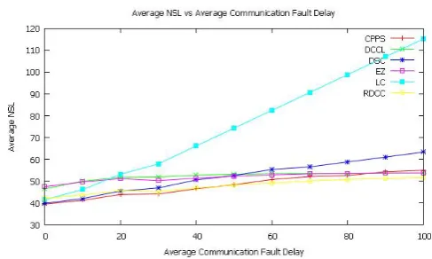
Fig. 1. Average NSL vs average communication fault delay for constant communication fault delay. The average percentage

variation order of NSL is:

EZ < DCCL < RDCC < CP P S < DSC < LC.

Figure 1 shows the average NSL vs average communication fault delay for constant communication fault delay. Average per-centage variation of NSL for CPPS ranges from 0.000000 to 39.339941 with an average of 21.689623. Average percentage variation of NSL for DCCL ranges from

0.000000 to 15.701477 with an average of 12.238085. Average percentage variation of NSL for DSC ranges from 0.000000 to 59.248132 with an average of 30.824493. Average percentage variation of NSL for EZ ranges from 0.000000 to 13.166381 with an average of 9.015570. Average percentage variation of NSL for LC ranges from 0.000000 to 178.140955 with an av-erage of 82.813149. Avav-erage percentage variation of NSL for RDCC ranges from 0.000000 to 22.822389 with an average of 13.321739. The average percentage variation order of NSL is:

Fig. 2. Average number of processors used vs average communication fault delay for constant communication fault delay.

The average percentage variation order of average number of processors used is:

CP P S < DCCL < EZ < DSC < RDCC < LC.

percentage variation of number of processors used by EZ ranges from -53.551913 to 0.000000 with an average of -39.095877. Average percentage variation of number of processors used by LC ranges from 2.888889 to 0.000000 with an average of -2.181818. Average percentage variation of number of processors used by RDCC ranges from -22.404372 to 0.000000 with an av-erage of -14.356682. The avav-erage percentage variation order of average number of processors used is:CP P S < DCCL < EZ < DSC < RDCC < LC.

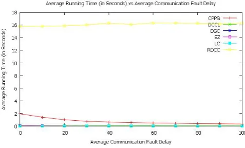
Fig. 3. Average running time (in seconds) vs average communication fault delay for constant communication fault delay. The average percentage variation order of average running time (in seconds) is:EZ < CP P S < DCCL < RDCC < DSC < LC.

Figure 3 shows the average running time (in seconds) vs average communication fault delay for constant communication fault de-lay. Average percentage variation of execution time for CPPS ranges from -83.545980 seconds to 0.000000 seconds with an average of -61.296417 seconds. Average percentage variation of execution time for DCCL ranges from -48.230505 seconds to 0.000000 seconds with an average of -32.104530 seconds. Av-erage percentage variation of execution time for DSC ranges from -7.494572 seconds to 23.195832 seconds with an average of 7.153515 seconds. Average percentage variation of execution time for EZ ranges from -84.616829 seconds to 0.000000 sec-onds with an average of -69.172067 secsec-onds. Average percentage variation of execution time for LC ranges from 0.000000 seconds

to 104.359697 seconds with an average of 45.954169 seconds. Average percentage variation of execution time for RDCC ranges from 0.000000 seconds to 3.283782 seconds with an average of 1.987271 seconds. The average percentage variation order of av-erage running time (in seconds) is:EZ < CP P S < DCCL < RDCC < DSC < LC.

Fig. 4. Average NSL vs average computation fault delay for constant computation fault delay. The average percentage variation

order of average NSL is:

EZ < LC < DCCL < DSC < RDCC < CP P S.

Figure 4 shows the average NSL vs average computation fault delay for constant computation fault delay. Average percentage variation of NSL for CPPS ranges from -56.728965 to 0.000000 with an average of -47.964772. Average percentage variation of NSL for DCCL ranges from -57.803176 to 0.000000 with an av-erage of -48.398015. Avav-erage percentage variation of NSL for DSC ranges from 57.064704 to 0.000000 with an average of -48.295160. Average percentage variation of NSL for EZ ranges from -61.778948 to 0.000000 with an average of -51.208754. Average percentage variation of NSL for LC ranges from -58.625609 to 0.000000 with an average of -49.596531. Average percentage variation of NSL for RDCC ranges from -57.411905 to 0.000000 with an average of -48.201589. The average percent-age variation order of averpercent-age NSL is:EZ < LC < DCCL < DSC < RDCC < CP P S.

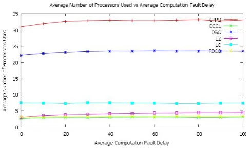
Fig. 5. Average number of processors used vs average computation fault delay for constant computation fault delay. The average percentage variation order of average number of processors used is:

Figure 5 shows the average number of processors used vs aver-age computation fault delay for constant computation fault de-lay. Average percentage variation of number of processors used by CPPS ranges from 0.000000 to 7.303974 with an average of 5.502392. Average percentage variation of number of processors used by DCCL ranges from 0.000000 to 18.750000 with an av-erage of 13.238636. Avav-erage percentage variation of number of processors used by DSC ranges from 0.000000 to 5.944319 with an average of 4.979821. Average percentage variation of number of processors used by EZ ranges from 0.000000 to 42.622951 with an average of 32.637854. Average percentage variation of number of processors used by LC ranges from -2.888889 to 0.000000 with an average of -2.181818. Average percentage variation of number of processors used by RDCC ranges from 0.000000 to 11.827957 with an average of 6.647116. The aver-age percentaver-age variation order of averaver-age number of processors used is:LC < DSC < CP P S < RDCC < DCCL < EZ.

Fig. 6. Average running time (in seconds) vs average computation fault delay for constant computation fault delay. The average

percentage variation order of running time (in seconds) is: RDCC < CP P S < DCCL < DSC < LC < EZ.

Figure 6 shows the average running time (in seconds) vs aver-age computation fault delay for constant computation fault de-lay. Average percentage variation of execution time for CPPS ranges from 0.000000 seconds to 7.643489 seconds with an aver-age of 5.144307 seconds. Averaver-age percentaver-age variation of execu-tion time for DCCL ranges from 0.000000 seconds to 9.347126 seconds with an average of 5.281630 seconds. Average percent-age variation of execution time for DSC ranges from -11.770253 seconds to 31.426996 seconds with an average of 11.020723 seconds. Average percentage variation of execution time for EZ ranges from 0.000000 seconds to 138.690877 seconds with an average of 99.486318 seconds. Average percentage variation of execution time for LC ranges from -18.176091 seconds to 83.926603 seconds with an average of 25.908160 seconds. Av-erage percentage variation of execution time for RDCC ranges from -7.079550 seconds to 0.000000 seconds with an average of -5.005273 seconds. The average percentage variation order of running time (in seconds) is:RDCC < CP P S < DCCL < DSC < LC < EZ.

Figure 7 shows the average NSL vs average computation com-munication fault delay for constant computation communica-tion fault delay. Average percentage variacommunica-tion of NSL for CPPS ranges from 47.284423 to 0.000000 with an average of -40.515767. Average percentage variation of NSL for DCCL ranges from 46.723321 to 0.000000 with an average of -39.927285. Average percentage variation of NSL for DSC ranges from -48.131674 to 0.000000 with an average of -41.121503.

Fig. 7. Average NSL vs average computation communication fault delay for constant computation communication fault delay. The

average percentage variation order of NSL is: DSC < RDCC < CP P S < LC < DCCL < EZ.

Average percentage variation of NSL for EZ ranges from -46.297128 to 0.000000 with an average of -39.482014. Aver-age percentAver-age variation of NSL for LC ranges from -46.719418 to 0.000000 with an average of -40.091101. Average percentage variation of NSL for RDCC ranges from -47.565465 to 0.000000 with an average of -40.565215. The average percentage varia-tion order of NSL is:DSC < RDCC < CP P S < LC < DCCL < EZ.

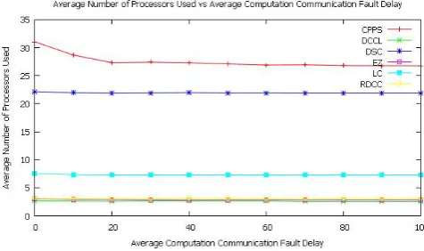
Fig. 8. Average number of processors used vs average computation communication fault delay for constant computation communication fault delay. The average percentage variation order

of number of processors used is:

CP P S < EZ < LC < DCCL < RDCC < DSC.

processors used by RDCC ranges from -3.743316 to 0.000000 with an average of -1.798736. The average percentage variation order of number of processors used is:CP P S < EZ < LC < DCCL < RDCC < DSC.

Fig. 9. Average running time (in seconds) vs average computation communication fault delay for constant computation communication fault delay. The average percentage variation order

of running time (in seconds) is:

EZ < CP P S < DCCL < RDCC < LC < DSC.

Figure 9 shows the average running time (in seconds) vs aver-age computation communication fault delay for constant compu-tation communication fault delay. Average percentage variation of execution time for CPPS ranges from -17.768162 seconds to 0.000000 seconds with an average of -13.567021 seconds. Av-erage percentage variation of execution time for DCCL ranges from -8.409209 seconds to 0.000000 seconds with an average of -6.374468 seconds. Average percentage variation of execution time for DSC ranges from 0.000000 seconds to 45.693766 sec-onds with an average of 23.202806 secsec-onds. Average percentage variation of execution time for EZ ranges from -22.443343 onds to 0.000000 seconds with an average of -17.522852 sec-onds. Average percentage variation of execution time for LC ranges from -5.702218 seconds to 53.187698 seconds with an average of 16.200082 seconds. Average percentage variation of execution time for RDCC ranges from -4.436490 seconds to 0.000000 seconds with an average of -3.309152 seconds. The average percentage variation order of running time (in seconds) is:EZ < CP P S < DCCL < RDCC < LC < DSC.

8. PERFORMANCE RESULTS FOR RANDOM FAULT DELAY

Figure 10 shows the average NSL vs average communication fault delay for random communication fault delay. Average per-centage variation of NSL for CPPS ranges from -57.657146 to 0.000000 with an average of -47.261227. Average percentage variation of NSL for DCCL ranges from -58.716447 to 0.000000 with an average of -47.870314. Average percentage variation of NSL for DSC ranges from -57.993719 to 0.000000 with an av-erage of -47.624933. Avav-erage percentage variation of NSL for EZ ranges from 62.491137 to 0.000000 with an average of -50.513271. Average percentage variation of NSL for LC ranges from -59.573872 to 0.000000 with an average of -48.991292. Average percentage variation of NSL for RDCC ranges from -58.371457 to 0.000000 with an average of -47.470166. The average percentage variation order of NSL is:EZ < LC < DCCL < DSC < RDCC < CP P S.

Figure 11 shows the average number of processors used vs aver-age communication fault delay for random communication fault

Fig. 10. Average NSL vs average communication fault delay for random communication fault delay. The average percentage

variation order of NSL is:

EZ < LC < DCCL < DSC < RDCC < CP P S.

Fig. 11. Average number of processors used vs average communication fault delay for random communication fault delay.

The average percentage variation order of number of processors used is:LC < DSC < CP P S < RDCC < DCCL < EZ.

delay. Average percentage variation of number of processors used by CPPS ranges from 0.000000 to 8.592911 with an av-erage of 5.556098. Avav-erage percentage variation of number of processors used by DCCL ranges from 0.000000 to 16.250000 with an average of 13.295455. Average percentage variation of number of processors used by DSC ranges from 0.000000 to 6.772009 with an average of 5.171352. Average percent-age variation of number of processors used by EZ ranges from 0.000000 to 49.726776 with an average of 35.022355. Average percentage variation of number of processors used by LC ranges from -4.000000 to 0.000000 with an average of -1.434343. Av-erage percentage variation of number of processors used by RDCC ranges from 0.000000 to 10.752688 with an average of 7.429130.The average percentage variation order of number of processors used is:LC < DSC < CP P S < RDCC < DCCL < EZ.

Fig. 12. Average running time (in seconds) vs average communication fault delay for random communication fault delay.

The average percentage variation order of running time (in seconds) is:RDCC < DCCL < CP P S < DSC < LC < EZ.

-1.464375 seconds to 58.513965 seconds with an average of 27.081776 seconds. Average percentage variation of execution time for EZ ranges from 0.000000 seconds to 141.977298 sec-onds with an average of 100.551805 secsec-onds. Average percent-age variation of execution time for LC ranges from -1.270763 seconds to 137.433058 seconds with an average of 44.802660 seconds. Average percentage variation of execution time for RDCC ranges from -6.555553 seconds to 0.000000 seconds with an average of -4.966295 seconds. The average percentage varia-tion order of running time (in seconds) is:RDCC < DCCL < CP P S < DSC < LC < EZ.

Fig. 13. Average NSL vs average computation fault delay for random computation fault delay. The average percentage variation

order of NSL is:

EZ < LC < DCCL < DSC < RDCC < CP P S.

Figure 13 shows the average NSL vs average computation fault delay for random computation fault delay. Average percentage variation of NSL for CPPS ranges from -55.454729 to 0.000000 with an average of -46.252097. Average percentage variation of NSL for DCCL ranges from -56.456555 to 0.000000 with an av-erage of -47.014353. Avav-erage percentage variation of NSL for DSC ranges from 55.813059 to 0.000000 with an average of -46.628080. Average percentage variation of NSL for EZ ranges from -59.497232 to 0.000000 with an average of -49.695130. Average percentage variation of NSL for LC ranges from -57.369522 to 0.000000 with an average of -48.036695. Average percentage variation of NSL for RDCC ranges from -55.916115

to 0.000000 with an average of -46.586764. The average per-centage variation order of NSL is:EZ < LC < DCCL < DSC < RDCC < CP P S.

Fig. 14. Average numbeer of processors used vs average computation fault delay for random computation fault delay. The average percentage variation order of number of processors used is:

LC < DSC < CP P S < RDCC < DCCL < EZ.

Figure 14 shows the average numbeer of processors used vs av-erage computation fault delay for random computation fault de-lay. Average percentage variation of number of processors used by CPPS ranges from 0.000000 to 7.035446 with an average of 5.438922. Average percentage variation of number of processors used by DCCL ranges from 0.000000 to 18.750000 with an av-erage of 13.295455. Avav-erage percentage variation of number of processors used by DSC ranges from 0.000000 to 6.245297 with an average of 4.897736. Average percentage variation of number of processors used by EZ ranges from 0.000000 to 49.180328 with an average of 34.923000. Average percentage variation of number of processors used by LC ranges from -2.666667 to 0.444444 with an average of -1.070707. Average percentage variation of number of processors used by RDCC ranges from 0.000000 to 10.695187 with an average of 6.757414. The aver-age percentaver-age variation order of number of processors used is:

LC < DSC < CP P S < RDCC < DCCL < EZ.

Fig. 15. Average running time (in seconds) vs average computation fault delay for random computation fault delay. The average

percentage variation order of running time (in seconds) is: RDCC < DSC < LC < DCCL < CP P S < EZ.

Average percentage variation of execution time for CPPS ranges from 0.000000 seconds to 14.814304 seconds with an average of 9.175700 seconds. Average percentage variation of execution time for DCCL ranges from 0.000000 seconds to 8.216433 sec-onds with an average of 5.047240 secsec-onds. Average percentage variation of execution time for DSC ranges from -21.159173 onds to 22.797506 seconds with an average of -2.713131 sec-onds. Average percentage variation of execution time for EZ ranges from 0.000000 seconds to 139.845090 seconds with an average of 98.640647 seconds. Average percentage variation of execution time for LC ranges from -38.532273 seconds to 49.750831 seconds with an average of 0.479462 seconds. Av-erage percentage variation of execution time for RDCC ranges from -7.767776 seconds to 0.000000 seconds with an average of -5.753271 seconds. The average percentage variation order of running time (in seconds) is:RDCC < DSC < LC < DCCL < CP P S < EZ.

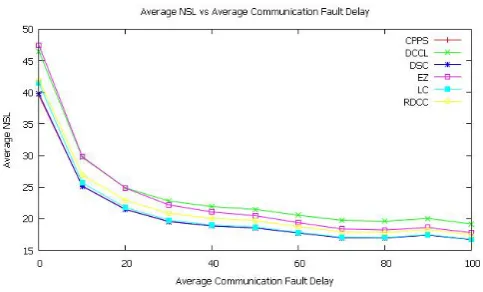
Fig. 16. Average NSL vs average computation communication fault delay for random computation communication fault delay.

The average percentage variation order of NSL is: EZ < LC < DCCL < DSC < RDCC < CP P S.

Figure 16 shows the average NSL vs average computation communication fault delay for random computation commu-nication fault delay. Average percentage variation of NSL for CPPS ranges from -57.344482 to 0.000000 with an average of -47.993664. Average percentage variation of NSL for DCCL ranges from 58.097523 to 0.000000 with an average of -48.496198. Average percentage variation of NSL for DSC ranges from -57.701895 to 0.000000 with an average of -48.339627. Average percentage variation of NSL for EZ ranges from -62.333172 to 0.000000 with an average of -51.220358. Aver-age percentAver-age variation of NSL for LC ranges from -59.291658 to 0.000000 with an average of -49.722045. Average percentage variation of NSL for RDCC ranges from -57.842815 to 0.000000 with an average of -48.072150. The average percentage variation order of NSL is:EZ < LC < DCCL < DSC < RDCC < CP P S.

Figure 17 shows the average number of processors used vs aver-age computation communication fault delay for random compu-tation communication fault delay. Average percentage variation of number of processors used by CPPS ranges from 0.000000 to 7.089151 with an average of 5.385216. Average percentage variation of number of processors used by DCCL ranges from 0.000000 to 18.125000 with an average of 12.670455. Aver-age percentAver-age variation of number of processors used by DSC ranges from 0.000000 to 7.072987 with an average of 5.260278. Average percentage variation of number of processors used by EZ ranges from 0.000000 to 46.448087 with an average of

Fig. 17. Average number of processors used vs average computation communication fault delay for random computation communication fault delay. The average percentage variation order

of number of processors used is:

LC < DSC < CP P S < RDCC < DCCL < EZ.

33.184302. Average percentage variation of number of proces-sors used by LC ranges from -3.555556 to 0.000000 with an av-erage of -1.878788. Avav-erage percentage variation of number of processors used by RDCC ranges from 0.000000 to 11.891892 with an average of 8.157248. The average percentage varia-tion order of number of processors used is:LC < DSC < CP P S < RDCC < DCCL < EZ.

Fig. 18. Average running time (in seconds) vs average computation communication fault delay for random computation communication fault delay. The average percentage variation order

of running time (in seconds) is:

RDCC < DCCL < CP P S < DSC < LC < EZ.

average of 17.828406 seconds. Average percentage variation of execution time for RDCC ranges from -7.048315 seconds to 0.000000 seconds with an average of -5.005104 seconds. The average percentage variation order of running time (in seconds) is:RDCC < DCCL < CP P S < DSC < LC < EZ.

9. CONCLUSION

Experiments mentioned in this paper were performed to iden-tify the task scheduling algorithms that also performs well in the presence of communication fault delay or computation fault de-lay. Six algorithms (CPPS, DCCL, DSC, EZ, LC, RDCC) were evaluated for two types of task graphs (i) task graphs with ran-dom fault delay and (ii) task graphs with constant fault delay. From the above graphs and results it can be concluded that for a constant communication delay EZ algorithm gives best result and LC algorithm as the worst result.This may be because EZ algorithm gives non linear clustering and LC algorithm gives linear clustering. RDCC algorithm performs good in the case of random delay.This may be because RDCC is a randomized algorithm. For future work other different problems like matrix multiplication and Gaussian elimination task graphs may be con-sidered and observed how it performs in the presence of faults.

10. REFERENCES

[1] Anil Kumar Tripathi, P.K. Mishra, Abhishek Mishra,Kamal sheel Mishra, Benchmarking the clustering algorithms for multiprocessor environments using dynamic priority of modules, Elsevier Applied Mathematical Modelling 36 (2012) 6243-6263.

[2] Alexey Lastovetsky, Parallel testing of Distributed Soft-ware, Elsevier Information and Software technology Vol 47 (2005) 657-662.

[3] Cyril Briquet, Reproducible testing of Distributed soft-ware with middlesoft-ware virtualization and simulation, ACM (2008).

[4] Giovanni denaro, Andrea polini, Wolfgang Emmerich, Early performance testing of distributed software applica-tions, ACM (2004).

[5] james D. Herbsleb, Audris Mockus, An Empirical study of speed and communication in globally distributed soft-ware development, IEEE transactions on softsoft-ware enginer-ing Vol 29 no. 6 (2003) june 481-494.

[6] raul cretta nunes, Ingrid jansch-porto, Modeling communi-cation delays in distributed systems using time series, IEEE transactions (2002) 268-273.

[7] Yizheng yao, Yingxu Wang, A framework for testing dis-tributed software components, IEEE transactions (2005) 1566-1569.

[8] Roger Ferguson, Bogdan Korel, Generating test data for distributed software using the chaining approach, Elsevier Information and software technology Vol 38 (1996) 343-353.

[9] Carl K. Chang, Cheng-Chung Song,Rong-Fa Wang, dis-tributed Software Testing with Specification, IEEE 1990. [10] Y. K. Kwok, I. Ahmad, Benchmarking and comparison of

the task graph scheduling algorithms, Journal of Parallel and Distributed Computing 59 (1999) 381–422.

[11] Kequin Li, Scheduling parallel tasks on multiprocessor computers with efficient power management, IEEE trans-actions (2010) 978-1-4244-6534, New York, USA. [12] john A. Stankovic, K. Ramamritham, S.Cheng, Evaluation

of a Flexible task scheduling algorithm for distributed hard real time systems, IEEE Transactions on Computers Vol c-34 , no. 12 (1985) 1130–1143.

[13] V.S. Tondre, V.M.Thakare, S.S.Sherekar, R.V. Dharaskar, Technical computation and communication delay in dis-tributed system, NCICT (2011) IJCA.

[14] R.C.Nunes,I.J. Porto, Modeling communication delays in distributed systems using time series, IEEE transactions (2002) 1060-9857/02, Brazil.

[15] P.K. Mishra, K.S. Mishra, A. Mishra, A clustering heuris-tic for multiprocessor environments using computation and communication loads of modules, International Journal of Computer Science & Information Technology, 2(5):170– 182, 2010.

[16] T.H. Cormen, C.E. Leiserson, R.L. Rivest, C. Stein, Intro-duction to Algorithms, 2nd Edition, MIT Press, 2001. [17] E. Horowitz, S. Sahni, Fundamentals of Computer

Algo-rithms, W. H. Freeman and Co., 1978.

[18] Y. Langsam, M.J. Augenstein, A.M. Tenenbaum, Data Structures Using C and C++, 2nd edition, Prentice Hall, 1996.

11. AUTHOR’S PROFILE

Anil Kumar Tripathiis Professor of Computer Engineering at Indian Institute of Technology (Banaras Hindu University), Varanasi, India. He received his Ph.D. degree in Computer Sci-ence from the same institute; and M.Sc. Engg. (Computer) de-gree from Odessa National Polytechnic University, Ukraine. His research interests include parallel and distributing computing, and software engineering.He has to his credit more than 50 re-search papers in International journals. He has co-authored two research monographs: one from Springer USA and other from John Wiley USA. Fourteen students have completed their Ph.D under his supervision.