Sparse Matrix based Computational Overhead Reduction in UMRT for N a power of 2

(1)

Sparse Matrix based Computational Overhead

Reduction in UMRT for N a power of 2

Preetha Basu,

Dept. of ECE, TKM College of Engineering,

Kollam, Kerala, India

R. Gopikakumari

Division of Electronics, SOE

Cochin University of Science and Technology Kochi, Kerala, India

ABSTRACT

Unique Mapped Real Transform (UMRT) is a transform which helps in frequency domain analysis of signals in the real domain. Different algorithms are developed for the computation of the unique MRT coefficients for N a power of 2 and for N an even number. They identify and place the UMRT coefficients in the form of an

N



N

UMRT matrix. The basis matrices of this transform are observed to be sparse in nature. In this paper a new technique is proposed to reduce the computational overhead in UMRT, the size N being a power of two, exploiting the sparse nature of the basis matrices

.

General Terms

Frequency domain analysis, Sparse representation.

Keywords

UMRT, Basis matrix, Frequency domain analysis, Sparse Basis Matrix.

1. INTRODUCTION

Transform theory plays a fundamental role in signal and image processing. A transform maps data into a different mathematical space via a transformation equation [1]. Analysis of the properties of the signal is easier with the transform of that signal. Discrete Fourier Transform (DFT) is an important tool in signal processing applications to map data from time domain to frequency domain [2]. FFT is the most popular algorithm to implement DFT which is highly efficient for 1-D signals. In most of the algorithms for DFT implementation, the input data will generally be real valued which is converted to complex form and the computations are done in complex domain. 2_D Mapped Real Transform (2-D MRT), evolved from 2-D Discrete Fourier Transform (2-D DFT), maps 2-D data into frequency domain without any complex operations but in terms of real additions alone [3]. Originally, the transform mapped a NNdata matrix into M redundant matrices of sizeNN, M=N/2. Algorithms were developed to identify and place, the unique MRT coefficients present in the M matrices for N a power of 2 or for N an even number, in the form of an

N



N

UMRT matrix. In [3], all the MRT coefficients are computed, the unique coefficients are identified and arranged in an

N



N

matrix whereas in [4] the basic DFT coefficients are identified and the corresponding MRT coefficients are computed and placed them in an NN UMRT matrix.

These algorithms are effectively utilized for image compression applications [5] and for texture studies [6]. The algorithm in [7] computes and places the UMRT coefficients directly from the data, without computing MRT.

The Haar transform is another signal transform that converts real input to real output, and has been used extensively in signal and image processing. MRT is a recently developed transform which also uses the real-to-real conversion property of the Haar transform. Relationships between these two transforms are studied in [8]. MRT is shown to have directional properties which is utilised for orientation estimation. A subset of global patterns of a 16x16 MRT is used to estimate the orientation field of fingerprint images[9]. Discrete transforms are performed based on specific functions, called the basis functions [2]. The discrete version of 2-D basis function is called basis matrices (or basis images). The process of transforming the image data into another domain involves projecting the image onto the basis images. The mathematical term for this projection process is called an inner product. A new technique is proposed in this paper to reduce the computational overhead in UMRT exploiting the sparse nature of the basis matrices.

2. 2-D Unique Mapped Real Transform

(2-D UMRT)

Let xn1,n2 , 0n1,n2N1 be the elements of

N

N data matrix. The 2-D MRT coefficients

Y

_kp₁_,k₂, are expressed as [3]



    





M p z ) ,n (n

,n n p

z ) ,n (n

,n n p

,k

k

x

Y

| 2 1

2 1 |

2 1

2 1 2

1

where 0k1,k2N1, 0 pM 1

(2)

p

z



or z pM and placed in the position

) N m))) .co_prime( ,((k N m))) .co_prime( (((k u u 2 1 ) , ( 1 2 

3. COMPUTATIONAL OVERHEAD IN

2-D UMRT

In most of the existing transforms like Walsh-Hadamard, Haar, DFT etc., all the input data contribute to each transform coefficient. The visual representation of MRT coefficients [8] shows that the actual computation of a UMRT coefficient involves selected set of data only. The actual number of input data participating in the computation of a particular UMRT coefficient Yu1,u2 in terms of addition/subtraction is given by 2.N.dm where dmg c d (k1,k2.M), divisor of M. There are N2 UMRT coefficients and hence a total of 2N3.dm addition/subtraction of data elements are involved in a UMRT computation. But the position of the data, to be added or subtracted, is identified by computing the parameter

N )) k n k ((n

z 1 1 2 2 _{and verifying whether its value} is p or p+M. Thus z is to be calculated N2 times to compute a particular UMRT coefficient even though only 2.N.dm data are involved. This causes an overhead in UMRT computation. Computational overhead can be reduced by exploiting the properties present in visual pattern of UMRT coefficients.

3.1 Interpretation using basis matrix

The UMRT computation can be represented as

The mapping between data and UMRT is many to many. The basis matrices for mapping the data to UMRT coefficients show sparse nature. Since the UMRT computation involves computational overhead due to the parameter z, the concept of basis matrix is introduced here to reduce the overhead.

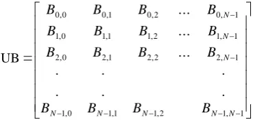
Basis matrix(UB), given below in matrix form, transforms the 2-D input data matrix to the transform domain.

UB

=













        1 , 1 2 , 1 1 , 1 0 , 1 1 , 2 2 , 2 1 , 2 0 , 2 1 , 1 2 , 1 1 , 1 0 , 1 1 , 0 2 , 0 1 , 0 0 , 0

.

...

N N N N N N N N

B

1 1 1 1 1 0 -1 0 1 -1 1 -1 0 1 0 -1

1 1 1 1 1 0 - 1 0 1 -1 1 -1 0 1 0 -1

1 1 1 1 1 0 -1 0 1 -1 1 -1 0 1 0 -1

0 0 0 0 0 -1 0 1 0 0 0 0 -1 0 1 0

-1 -1 -1 -1 -1 0 1 0 -1 1 -1 1 0 -1 0 1

0 0 0 0 0 1 0 -1 0 0 0 0 1 0 -1 0

1 1 1 1 1 0 -1 0 1 -1 1 -1 0 1 0 -1

-1 -1 - 1 - 1 -1 0 1 0 -1 1 -1 1 0 -1 0 1

1 1 1 1 1 0 -1 0 1 -1 1 -1 0 1 0 -1

-1 -1 -1 -1 -1 0 1 0 -1 1 -1 1 0 -1 0 1

0 0 0 0 1 0 -1 0 0 0 0 0 0 1 0 -1

1 1 1 1 0 1 0 -1 1 -1 1 -1 1 0 -1 0

0 0 0 0 -1 0 1 0 0 0 0 0 0 -1 0 1

[image:2.595.322.507.225.316.2]

-1 -1 -1 -1 0 -1 0 1 -1 1 -1 1 -1 0 1 0

Figure 1: Basis matrices of 4-point 2-D UMRT

Each element Bu1,u2 in UB is a basis matrix of size NxN corresponding to the UMRT coefficient Yu1,u2. The elements bn1,n2 of the basis matrix Bu1,u2 is given by

𝑏𝑛1,𝑛2=

1, 𝑖𝑓 𝑧 = 𝑝 −1, 𝑖𝑓 𝑧 = 𝑝 + 𝑀

0, 𝑒𝑙𝑠𝑒

3.2 Number of non-zero elements in the

Basis matrix B

u1,u2.

The 2-D MRT coefficient

p ,k k

Y1 2_{maps the N x N data}

matrix onto p twiddle factor axes in the frequency domain[2]. The number of p values depends on the frequency index (k1,k2) and is given by N/2dm or M/dm. The total number of elements in basis matrix

2 2 ,

1 N

Bu u  . The number of p values =M/dm.

The total number of non-zero elements in basis matrix Bu1, u2 = N2 ÷ M /dm= 2.N.dm

(3)

When N = 8 and k1=0, k2=0, dm=gcd(0,0,4)=4 and M/dm=1. Thus p has only one value, that is p=0. Since p has only one value that is zero, all the 64 inputsamples are mapped onto p=0 axis and hence elements of basis matrix B0,0 are all 1.

When N = 8 and k1=0, k2=1, dm=gcd(0,1,4)=1 and M/dm=4 , p has 4 values, ie p=0,1,2,3. Since p has four values, 64 input samples of xn1,n2 are divided in 4 groups of 16 each. Correspondingly the basis matrix B 0, 1 and three other associated basis matrices will have sixteen non-zero elements each.

4. Modified

algorithm

for

UMRT

computation exploiting sparse basis

matrix.

The algorithm is developed based on the observation of the patterns present in the visual representation of MRT coefficients and basis matrices of UMRT coefficients. Initially, the row and column indices (n1,n2)of non-zero basis elements are identified for computing a particular UMRT coefficient. Data elements xn1,n2 in those positions are added together without computing z. The sign of xn1,n2 can be found from

−1( 𝑛1𝑘1+𝑛2𝑘2 −𝑝 ) 𝑁_{. Although the sparse nature of} basis matrix is exploited, there is no need to create a basis matrix in the present implementation. The transform coefficients are categorized into three as

0

2 ,

0

1 

k



k

and others.

When k10,all the rows of the basis matrix has elements. Since there are 2N.dmnon-zero elements in a basis matrix, each row has 2N.dm/N 2dm elements. The row index is incremented by

2 dm

from 0 to N. Thus 2N.dm row indices are formed. Column index occurs in an increment of N/2dm in the interval 0 to N and is repeated N times for N rows. Thus NN/2dm is repeated N times which is equal to 2N.dm column indices. It is seen from

inspection that when p increases column index is incremented once. For different p’s, each column index is incremented by p/dm times. Row index is retained as such.

When k20, all the columns of the basis matrix has elements. The column index is incremented by

2 dm

from 0 to N. Thus 2N.dm column index is formed. Row index is incremented from 0 to N in steps of

dm

N/2 and is repeated N times. That is NN/2dmis repeated N times which is equal to 2N.dmcolumn indices. For different p’s, each row index is incremented by p/dmtimes. Column index is retained as such.

When k1&k2not equal to zero, the row index is incremented from 0 to N , 2dm times. Thus

dm N.

2 row indices are formed. Column index is incremented from 0 to N in steps of N/2dmk2, where dmk2 is

gcd(

M

,

k

2 )

and is repeated

2 / .dm dmk

N times. Thus

2 2 / 2 /

.dm dmk N dmk

N  is repeated N times

which is equal to 2N.dmcolumn indices. From the visual representation of basis matrices it is seen that, with each increment in p, the row and column indices are incremented in a special pattern. For different p’s, each row index is incremented by p.r/dm times, each column index is decremented by p.c/dm times. Constant r and c depends on the coefficients k1,k2 and satisfies the equations, ((𝑘1. 𝑟))𝑘2= 𝑑𝑚 and 𝑘1. 𝑟 = 𝑑𝑚 +

𝑘2. 𝑐.

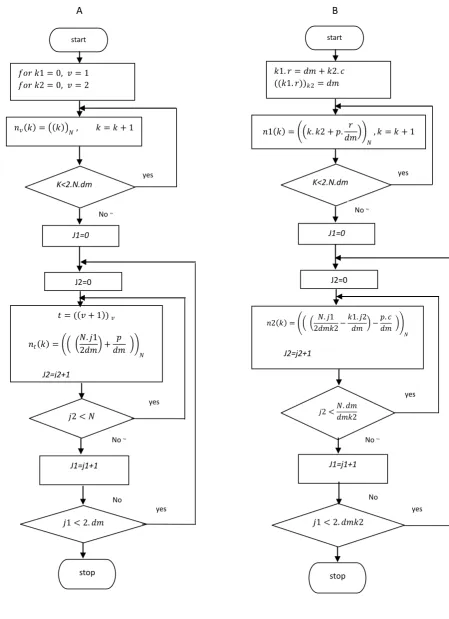
Various steps involved in the algorithm are depicted using a Flow Chart in figure 3. The sub processes of finding out the row and column indices of sparse basis matrices for various (k1,k2) (Block A and block B ) are

(4)

A

Find row and column index

Identify the index basic DFT coefficients ,D

start

N, M=N/2, YN,N

div_M={0,divisors ofM} w=1, D (3N-2),2 =0

D(w)=(k1,k2) , w=w+1

dm=gcd(k1,k2,M) , m=0

Co_prime(m)=2m+1 P=m*dm , k=0

(k1 , k2)

w>3N-2

𝑚 ≥ 𝑀/𝑑𝑚 𝑌 𝑢1, 𝑢2 = 𝑌(𝑘1. 𝑐𝑜_𝑝𝑟𝑖𝑚𝑒 𝑝

𝑑𝑚 , 𝑘2. 𝑐𝑜_𝑝𝑟𝑖𝑚𝑒 𝑝 𝑑𝑚 )

𝑌 _𝑘1,𝑘2𝑝 = −1( 𝑛1.𝑘1+𝑛2.𝑘2 −𝑝 ) 𝑁 𝑛1,𝑛2

𝑥 𝑛1,𝑛2

m=m+1

stop

B

Find row and column index

K1=0/k2 =0 K1,k2 =others

=0

No

Yes

No

[image:4.595.163.420.62.763.2]

(5)

stop

start

J1=0

𝑛1 𝑘 = 𝑘. 𝑘2 + 𝑝. 𝑟

𝑑𝑚 _𝑁, 𝑘 = 𝑘 + 1

𝑛2 𝑘 = 𝑁. 𝑗1 2𝑑𝑚𝑘2−

𝑘1. 𝑗2 𝑑𝑚 −

𝑝. 𝑐 𝑑𝑚

𝑁

J2=j2+1

J2=0

K<2.N.dm

𝑗2 <𝑁. 𝑑𝑚 𝑑𝑚𝑘2

𝑗1 < 2. 𝑑𝑚𝑘2

J1=j1+1

𝑘1. 𝑟 = 𝑑𝑚 + 𝑘2. 𝑐 ((𝑘1. 𝑟))𝑘2= 𝑑𝑚

yes

Yes

yes

Yes

NoYes

No

Yes

yes

Yes

NoYes

stop

start

J1=0

𝑛𝑣 𝑘 = 𝑘 _𝑁 , 𝑘 = 𝑘 + 1

𝑡 = ( 𝑣 + 1 ) 𝑣

𝑛𝑡 𝑘 =

𝑁. 𝑗1 2𝑑𝑚 +

𝑝 𝑑𝑚 _𝑁

J2=j2+1

J2=0

K<2.N.dm

𝑗2 < 𝑁

𝑗1 < 2. 𝑑𝑚

J1=j1+1

𝑓𝑜𝑟 𝑘1 = 0, 𝑣 = 1 𝑓𝑜𝑟 𝑘2 = 0, 𝑣 = 2

yes

Yes

yes

Yes

NoYes

No

Yes

yes

Yes

NoYes

[image:5.595.98.548.78.698.2]

A

B

(6)

The Algorithm

1. Initialize 𝑁, 𝑀 = 𝑁/2, 𝑌𝑁,𝑁= 0 find divisors of M, div_m={0 and divisors of M}.

2. Identify frequency indices

(

k

1 ,

k

2 )

of basic DFT coefficients.

3. Find p’s for each

(

k

1 ,

k

2 )

4. For each

(

k

1 ,

k

2 ,

p

)

, find row and column indices (n1 and n2) of xn1,n2added to find 𝑌𝑢1,𝑢2

5. The transform coefficients

𝑌 𝑘1,𝑘2𝑝 = −1 𝑛1.𝑘1+𝑛2.𝑘2 −𝑝 𝑁 𝑛1,𝑛2

𝑥 𝑛1,𝑛2

6. UMRT coefficients

𝑌 𝑢1, 𝑢2 = 𝑌 𝑘1. 𝑐𝑜_{𝑝𝑟𝑖𝑚𝑒}𝑝

𝑑𝑚 , 𝑘2. 𝑐𝑜𝑝𝑟𝑖𝑚𝑒 𝑝 𝑑𝑚

5. RESULTS AND ANALYSIS

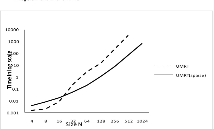
[image:6.595.339.552.101.350.2]

The proposed algorithm for the UMRT computation is implemented on Intel core i5 machine with clock speed 2.4 GHz and 4GB RAM. Lena image is used to compare the performance of the present algorithm with the previous algorithm[7]. The table I shows the results of comparison performed. A sharp increase of computational time saving is attained for different values N. Fig 4 gives a graphical representation of the comparison made, time being in logarithmic scale.

Figure 4: Graph showing comparison of time taken in log scale as a function of N.

TABLEI:TIME TAKEN FOR UMRT COMPUTATION

Size N

Computation time (sec)

UMRT UMRT(sparse)

4 0.0014 0.0035

8 0.0019 0.0070

16 0.0073 0.0163

32 0.2112 0.0480

64 2.5972 0.1745

128 14.32 1.02

256 193.21 7.44

512 3123.11 62.22

1024 _ 642.70

0.001 0.01 0.1 1 10 100 1000 10000

4 8 16 32 64 128 256 512 1024

UMRT

UMRT(sparse)

Tim

e

in

lo

g

sca

le

[image:6.595.99.473.482.707.2]

(7)

6. CONCLUSION

The result shows a considerable amount of saving in time especially when the size of the data matrix increases. The proposed algorithm is faster compared to the earlier algorithms. Although the computation time is comparable or slightly higher for small values of N, as N increases the sparse matrix method of implementation performs exceedingly faster.

Thus if the UMRT computation exploiting the sparsity of basis matrices proposed in this paper is used in frequency domain analysis of 2-D signals, especially for applications like video processing and image enhancement where size of the image taken is large, the computation time will be drastically reduced. An alternate placement approach for arranging the unique MRT coefficients in the order of sequencies is proposed in [11] named as SMRT. Since the basis matrices are the same, the proposed algorithm can be used to reduce the computational complexity of SMRT computation also.

7. REFERENCES

[1] A K Jain, “Fundamentals of digital image processing”, Prentice Hall New Delhi, India, 2003.

[2] Alexander D. Poularikas, “Transforms and Applications Handbook”, Third Edition,CRC press, 2010.

[3] Rajesh Cherian Roy and R. Gopikakumari “A new transform for 2-D signal representation (MRT) and some of its properties”, 2004 IEEE International Conference on Signal Processing and Communications.

[4] Bhadran. V, R.C.Roy, R.Gopikakumari, “Algorithm to identify basic coefficients of 2-D DFT for any even N”. in proc. ICVCOM, Saintgits college of engineering,Kottayam,Apr 16-18,2009.

[5] M. S. Anish Kumar, Rajesh Cherian Roy and R. Gopikakumari, “A new image compression and decompression technique based on 8x8 MRT”, International Journal on Graphics, Vision and Image Processing, Volume 6, July 2006, pp. 51-53 .

[6] Meenakshy K., “Development & Implementation of a CAD System to predict the Fragmentation of Renal Stones Based on Texture Analysis of CT Images”, Ph. D Dissertation, Cochin University of Science & Technology, Kochi, 2010.

[7] Preetha Basu, Bhadran.v., Gopikakumari.R, “A new algorithm to compute forward and inverse 2-D UMRT for N — A power of 2”,IEEE International Conference on Power, Signals, Controls and Computation (EPSCICON), 2012 .

[8] Rajesh Cherian Roy and R. Gopikakumari “Relationship between the Haar transform and the MRT”, 8th

International Conference on Information, Communication and Signal processing(ICICS), 2011.

[9] Rajesh Cherian Roy and R. Gopikakumari, “A Transform(MRT) naturally suited for Directional Pattern Analysis”, Proc. SPIE8760, January 28, 2013.

[10]Bhadran. V, R. C. Roy, R. Gopikakumari, “Visual Representation of 2-D DFT in terms of 2x2 data, A pattern analysis”, proceedings of international conference on computing, communication and Networking (ICCCN ’08), Chettinad college of engineering and technology, karur, India, dec 18-20, 2008 .