An Innovative Approach for Attribute Reduction in Rough Set Theory

(1)

http://dx.doi.org/10.4236/iim.2014.65022

An Innovative Approach for Attribute

Reduction in Rough Set Theory

Alex Sandro Aguiar Pessoa, Stephan Stephany

National Institute for Space Research (INPE), Sao Jose dos Campos, Brazil Email: [email protected], [email protected]

Received 4 July 2014; revised 3 August 2014; accepted 25 August 2014

This work is licensed under the Creative Commons Attribution International License (CC BY). http://creativecommons.org/licenses/by/4.0/

Abstract

The Rough Sets Theory is used in data mining with emphasis on the treatment of uncertain or va-gue information. In the case of classification, this theory implicitly calculates reducts of the full set of attributes, eliminating those that are redundant or meaningless. Such reducts may even serve as input to other classifiers other than Rough Sets. The typical high dimensionality of current da-tabases precludes the use of greedy methods to find optimal or suboptimal reducts in the search space and requires the use of stochastic methods. In this context, the calculation of reducts is typ-ically performed by a genetic algorithm, but other metaheuristics have been proposed with better performance. This work proposes the innovative use of two known metaheuristics for this calcu-lation, the Variable Neighborhood Search, the Variable Neighborhood Descent, besides a third heuristic called Decrescent Cardinality Search. The last one is a new heuristic specifically pro-posed for reduct calculation. Considering some databases commonly found in the literature of the area, the reducts that have been obtained present lower cardinality, i.e., a lower number of attributes.

Keywords

Rough Set Theory, Reducts, Attribute Reduction, Metaheuristics

1. Introduction

(2)

These strong aspects of RST have helped to spread its use over the last years. A weak aspect of RST is the non availability of free RST software, except for limited implementations. On the other hand, there is RST proprie-tary software.

RST is an extension of the set theory and has the implicit feature of compressing the dataset. Such compres-sion is due to the definition of equivalence classes based on indiscernibility relations and to the elimination of redundant or meaningless attributes. A central concept in RST is attribute reduction, which generates reducts. A reduct is any subset of attributes that preserves the indiscernibility of the elements for the considered classes, al-lowing performing the same classification that would be obtained with the full set of attributes. This work fo-cuses on the calculation of reducts in RST, which is a NP-hard problem [2]. A brief outline of RST follows in Section 2, while attribute reduction for RST is approached in Section 3.

It is common to employ the RST as a way of preprocessing to obtain reducts for other machine learning tech-niques. The typical high dimensionality of current databases precludes the use of greedy methods imbedded in RST to find optimal or suboptimal reducts in the search space, requiring the use of stochastic methods. This is-sue is tackled by the use of metaheuristics, such as genetic algorithms to calculate reducts [3]. In this context, attribute reduction was approached by [4] which proposed some metaheuristics, such as Ant Colony and Simu-lated Annealing for reduct calculation in RST, besides a Genetic Algorithm. Results are shown for some known databases intended for classification. Tabu Search was also proposed in [5] and applied for the same databases. These former results can be taken as benchmarks. The present work evaluates alternative metaheuristics for re-duct calculation in RST, being applied for the classification of the same databases.

The alternative metaheuristics proposed here for reduct calculation are Variable Neighborhood Search (VNS) and Variable Neighborhood Decent (VND), and a new one (actually a heuristic) called Decrescent Cardinality Search (DCS) [6]. VNS and VND are well known [7]. VNS generates a random candidate solution (or reduct) with any cardinality and at every iteration explores its neighborhood searching for new solutions that are then evaluated. VND searches for solutions following a deterministic approach. It is an extension of VNS. On the other hand, DCS is a modified version of VNS that explores the search space aiming only at a lower cardinality reduct. It enforces randomly a cardinality reduction at each iteration before performing a local search. Section 4 describes VNS, VND and DCS. Local search was performed by a standard scheme or using VND itself. For the sake of simplicity, DCS is also denoted as a metaheuristic in the rest of this work.

In the scope of attribute reduction in RST applied to classification, any metaheuristic requires an evaluation function in order to rank the candidate solutions/reducts. Two different functions were evaluated in this work for the calculation of reducts in RST: the dependency degree between attributes and the relative dependency [8]. These functions, presented in Section 3.2, allows simplifying the calculation of the reducts in comparison with the standard approach based on the discernibility matrix, which presents high computational complexity, not being feasible for large and complex datasets. As mentioned above, three alternative metaheuristics are eva-luated for the calculation of reducts in RST: VNS, VND and DCS, which are described in Sections 4.1, 4.2 and 4.3, respectively. In addition, two local search schemes are also evaluated. Test results for some well- known databases are shown in Section 5. Processing time is also discussed. Each test case is related to the use of a spe-cific metaheuristic for the calculation of reducts applied to the classification of a spespe-cific database.

2. Rough Set Theory

Real world informations are often uncertain, vague or incomplete due to difficulties associated to record or re-port any natural phenomena or events that are under study. Some approaches are well known to tackle such is-sues, mainly the Fuzzy Set theory [9], the Dempster-Shafer theory [10] [11], and the possibility theory [12]. In the beginning of the eighties, another theory emerged for treating such kind of information, the Rough Set Theory-RST [1]. This theory is simple and has a good mathematical formalism. It is an extension of the set theory that deals with data uncertainty by means of an equivalence relation known as indiscernibility. Two ele-ments of a given set are considered as indiscernible if they present the same properties, according to a defined set of features, attributes or variables. Some authors like [13] point out that the main advantage of RST is not requiring additional informations such as the probability distribution, a priori probability or pertinence degree.

(3)

ele-ments in the set. On the other hand, in the RST, membership is not the primary concept. Rough sets represent a different mathematical approach to vagueness and uncertainty. Definition of a set in the RST is related to our information (knowledge) and perception about elements of the universe. It is based on the concept of indiscerni-bility: different elements can be discernible/indiscernible based on the information about them. Indiscernibility is defined as an equivalence relation that allows partitioning the universe into regions that express the classes that compose this universe.

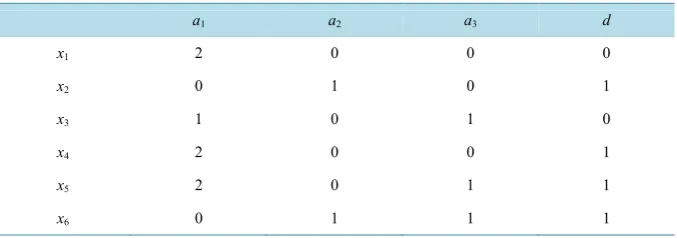
Although RST was proposed to deal with inconsistencies of information in the considered dataset, one of its main issues is to compact the dataset. This is achieved by means of eliminating elements with equal characteris-tics that are indiscernible in the sense that a unique element represents the others. A further way to compact the database is given by the reducts that eliminate redundant or meaningless attributes (superfluous attributes). A reduct is a subset of attributes that provides a classification with a minimum cardinality (minimum number of attributes) but still preserving the equivalence classes obtained with the full set of attributes. The concepts of in-discernibility and reducts help to reduce the volume of data [2]. In order to explain such basic concepts of RST in the next sections, an example dataset is shown inTable 1.

2.1. Indiscernibility Relations

In the RST, data are stored in a tabular format forming a pair S = (U; A) called an information system, where U is the non-empty set of elements/objects called universe and A is a finite set of conditional attributes such that a: U → Va for all a ∈ A. The set Va contains the possible values of attribute a. The elements of A are called condi-tional attributes or simply conditions. In order to perform a supervised learning, the addition of a decision attribute is required. The resulting information system is S=

(

U A; ∪

{ }

d

)

, where d ∉ A is the decision attribute. For the example shown in theTable 1, the universe is U = {x1, x2, x3, x4, x5, x6}, the set of conditional attributes is A = {a1, a2, a3} and the decision attribute is d. Possible values for the conditionals attributes values are: Va1 = {0, 1, 2} and Va2 = Va3 = {0, 1}. The decision attribute d allows definition of classes X1, , X| |Vd , where Vd ,

denotes the cardinality of its domain. In the example dataset, Vd =2, since Vd = {0, 1}. The corresponding

classes are X1 and X2, the first composed of elements with d = 0, and the second, of elements with d = 1.

RST provides the definition of an equivalence relation, which groups together elements that are indiscernible into classes, providing a partition of the universe of elements. Given an information system S = (U; A), and a subset of attributes B A⊆ , an equivalence relation INDA (B) is defined as follows (omitting the subscript A, it can be simplified to IND (B)):

( ) (

{

,

)

,

( )

} {

, x x2, 6

}

Table 1. An example dataset with three conditional attributes and one decision attribute.

a1 a2 a3 d

x1 2 0 0 0

x2 0 1 0 1

x3 1 0 1 0

x4 2 0 0 1

x x1, 4

} { } { } { } { }

, x2 , x3 , x5 , x6

}

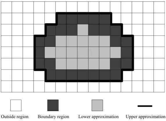
In the RST, these partitions based on an indiscernibility relation are called approximations (Figure 1) and al-low defining, for each class, four regions: al-lower approximation, upper approximations, boundary and outside re-gions. The lower approximation is composed of elements that certainly belong to the considered class, while the upper is composed of elements that possibly belong to it. The difference between the upper and the lower ap-proximations is the boundary region, while the outside region is composed of the elements that surely do not belong to the considered class. In the case of an empty boundary region, the dataset is called crisp, as in the tra-ditional data set theory. Otherwise, the dataset is said to be rough.

The outside and boundary regions can be obtained from the lower and upper approximations B-lower and B-upper for a considered class X, denoted respectively by BX and BX :

{

[ ]B

}

BX = x x ⊆X (2)

{

[ ]B

}

BX = x x ∩X ≠ ∅ (3) Elements contained in BX surely belong to class X, while the elements in BX can only be classified as possibly belonging to class X. The set FB=BX BX− is the boundary region of X, and its elements cannot de-cisively be assigned to class X. Finally, the set EB = −U BX is the outside region of class X, containing ele-ments that surely do not belong to this class.

Considering IND a a a

(

{ , , }1 2 3

)

for the example dataset, with its two classes X1 = {x1, x3} and X2 = {x2, x4, x5, x6}, the corresponding lower approximation

( )

BX , upper approximation

( )

BX , outside region (E) and boun-dary region (F) are:

{ }

1 3 ;

BX = x BX2=

{

{ } { } { }

x2 , x5 , x6

}

;

{

} { }

{

}

1 1, 4 , 3 ;

BX = x x x BX2=

{

{ }

x2 ,

{ }

x x1, 4 ,

{ } { }

x5 , x6

}

;

( )

1 1 1

{

1, 4

}

;

F X =BX BX− = x x F X

( )

2 =BX2−BX2=

{

x x1, 4

}

;

( )

1 1

{

{ } { } { }

2 , 5 , 6

}

.

F X = −U BX = x x x F X

( )

₂ = −U BX₂=

{ }

x₃ .

Another RST definition is the positive region for IND (B), denoted by POSB (d), that is the union of the lower

[image:4.595.171.457.501.709.2]

Outside region Boundary region Lower approximation Upper approximation

(5)

approximations of all classes, i.e. BX1∪ ∪ BX| |Vd .

2.2. Reducts

In RST, the size of the dataset can be reduced either by representing a whole class given by an indiscernibility relation (by means of a single element of this class) or by eliminating superfluous attributes that do not contri-bute to the classification. Given the original set A, a set B is called a reduct when INDA (B) = INDA (A), with

B A⊆ . Then, if B < A , where ⋅ denotes the cardinality of the set, this implies in an attribute reduction, but preserves the information contained in the data that is relevant for the classification. The total number reducts of a decision system with m attributes is given by all possible combinations of attributes, as given by [2]:

2 m m

 

 

 

 

 _{ }

 

(4)

where the term _m 2_ denotes the floor, the largest integer that is less or equal to m/2.

The calculation of reducts is a non-trivial task as reported by [2]. The simple increase of computational power does not allow the calculation of reducts for complex databases, since it constitutes a NP-hard problem for large and complex databases. This is a major performance bottleneck of the RST.Table 2 shows the number of possi-ble reducts for an m-attribute database according to Equation (4).

3. Attribute Reduction in Rough Set-Theory

Attribute reduction in RST implies in the calculation of the reducts. The classic approach is to obtain the discer-nibility matrix, to determine its correspondent discerdiscer-nibility function and to simplify it, in order to get the set of reducts. However, this approach is very expensive computationally, mainly for complex datasets. Another ap-proach that circumvents this problem is to formulate the calculation of reducts as an optimization problem that is iteratively solved by some metaheuristic. It requires the use of an evaluation or objective function in order to rank the reducts to choose the best candidate solution of the current iteration. Both approaches are detailed in the next sections.

3.1. Discernibility Matrix-Based Approaches

In these approaches, the calculation of reducts requires the discernibility matrix. For given information system S with n elements has a symmetric discernibility matrix with dimension n × n. The entries of this matrix are de-noted by cij, for i j≠ . Each entry contains the subset of attributes that distinguishes element xi from xj, being the diagonal entries null, according the definition below. The discernibility matrix for the example dataset is ap-pears inTable 3.

( )

{

}

ij i j

c = a A a x∈ ≠a x for i j, =1, , n and i j≠ (5)

The corresponding discernibility function fA is a Boolean function of m attributes

(

a a1, , ,2 am

)

, given by:

(

1, ,

)

{

1 ,

}

A n ij ij

[image:5.595.185.412.622.720.2]

f a∗ a∗ _{= ∧ ∨}c∗ _{≤ ≤ ≤}j i n c _{≠ ∅} ₍₆₎

Table 2. Number of possible reducts for a database with m attributes.

m # Possible Reducts

10 252

20 184,756

30 155,117,520

(6)

Table 3. Discernibility matrix for the example dataset.

x1 x2 x3 x4 x5 x6

x1 -

x2 a1, a2 -

x3 a1, a3 a1, a2, a3 -

x4 Ø a1, a2 a1, a3 -

x5 a3 a1, a2, a3 a1 a3 -

x6 a1, a2, a3 a3 a1, a2 a1, a2, a3 a1, a2 -

where cij∗=

{

a a c∗ ∈ ij

}

.

The Boolean simplification of fA yields the set of reducts of A, as follows. For the example dataset, the appli-cation of Equation (6) gives its discernibility function:

( ) (

) (

) ( ) (

)

(

) (

) ( )

(

) ( ) (

)

( ) (

)

(

)

a1 a2 a1 a3 a3 a1 a2 a3 a1 a2 a3 a1 a2 a1 a2 a3 a3

a1 a3 a1 a1 a2 a3 a1 a2 a3 a1 a2

f x =_ ∨ ∧ ∨ ∧ ∧ ∨ ∨ _{ } ∧ ∨ ∨ ∧ ∨ ∧ ∨ ∨ ∧ _

∧_ ∨ ∧ ∧ ∨  _{ }∧ ∧ ∨ ∨ _{ } ∧ ∨ _

Note that this logical function is expressed by the conjunction of many terms, with each one corresponding to a column of the related discernibility matrix. The Boolean simplification of this function yields then a single re-duct:

( )

a1 a3

f x = ∧

Therefore, this reduct is composed of attributes a1 and a3, and the original dataset shown inTable 1 can be represented in a shorter form without loss of information by a new table (Table 4).

3.2. Dependency Function-Based Approaches

In these approaches, a metaheuristic is employed to iteratively refine candidate solutions (reducts) that are ranked by an evaluation or objective function. A common choice for this function is the dependency function, employed in the Rough Set Attribute Reduction method (RSAR), exposed in Section 3.2.1. It measures the re-dundant information or dependency between a subset of conditional attributes and the decision attribute. If such a subset has a dependency degree equal or higher than the one of the complete set of attributes, then it is a poss-ible solution, i.e. it constitutes a reduct. However, it still presents high computational complexity, since it de-mands the calculation of the discernibility function and of the positive region for the considered solution. Alter-natively, the concept of relative dependency, presented in Section 3.2.2, provides an evaluation function with lower computational cost than the dependency degree. This work employs both evaluation functions for any of the proposed metaheuristics that were tested (VNS, VND and DCS).

3.2.1. Rough Sets Attribute Reduction (RSAR)

A most common approach for the calculation of reducts in RST is the Rough Set Attribute Reduction method (RSAR), that employs as evaluation function the dependency degree of rough sets [14] [15]. The dependency degree, defined in Equation (7), evaluates if a subset of attributes has redundant information in respect to anoth-er subset of attributes. Considanoth-ering two subsets of attributes, a subset B to be evaluated and a subset given by the decision attribute itself

( )

{ }

d , their corresponding indiscernibility relations in Uare IND (B) and IND d

( )

{ }

, respectively.

The dependency degree between B and

{ }

d is then defined as:

{ }

( )

B

( )

{ }

B

POS d

d

U

γ = (7)

(7)

[image:7.595.128.471.97.221.2]

Table 4. A reduced dataset considering a reduct with attributes a1 and a3.

a1 a3 d

x1 2 0 0

x2 0 0 1

x3 1 1 0

x4 2 0 1

x5 2 1 1

x6 0 1 1

{ }

( )

1

B d

γ < then

{ }

d depends partially on B. Finally, if γB

( )

{ }

d =0 then B does not depend on

{ }

d . The dependence degree between subsets of attributes minimizes inconsistencies in the information system, since it ranks a subset according to the redundancy of its attributes. The dependency degree between a subset and the decision attribute, shown above, allows calculating reducts. Considering the complete set of attributes A, any subset B such that γB

( )

{ }

d ≥γA

( )

{ }

d is a reduct. This can be proved as follows.

If B is a subset of the complete set of attributes A, then B A⊆ , and

{ }

d the set containing the decision attribute, then the set R of all possible reductions is given by:

{ }

( )

{ }

{

: B A

}

R= B B A⊆ γ d ≥γ d (8) In the example dataset, d = 0 determines class X1 = {x1, x4}, and d = 1, class X2 = {x2, x3, x5, x6}. Equation (7) yields the dependency degree of the full set of attributes A = {a1, a2, a3}:

{ }

( )

{ } { } { } { }

2 , 3 , 5 , 6 4 6 A

x x x x

d

U

γ = =

( )

{ }

2

6 a a d

γ =

Finally, subset {a1, a3} can be considered reduct, since it has dependency degree equal to A.

3.2.2. Attribute Reduction Based on Relative Attribute Dependency

A less computationally expensive way to evaluate a candidate solution (i.e. a reduct) is by means of an alterna-tive metric called relaalterna-tive dependency, proposed by [8] in the scope of the RST. The relative attribute depen-dency degree can be calculated by the ratio of the number of partitions of the universe for a considered subset of conditional attributes and the number of partitions for the union of such subset with the decision attribute. Given A, the set of all conditional attributes, B A⊆ and

{ }

d the decision attribute, the relative dependency is given by:

{ }

( )

₍

( )

_{{ }}

₎

B

U IND B d

κ =

∪ (9)

Employing the relative dependency κB instead of the dependency degree γB in Equation (8) also yields the set of reducts:

{ }

( )

{ }

{

: B A

}

(8)

{ }

( )

_{{ } { } { } { } { } { }}

{

1 4

} { } { } { } { }

2 3 5 6

1 2 3 4 5 6

, , , , , ₅

6

, , , , ,

A

x x x x x x

d

x x x x x x

κ = =

Repeating the calculation of κB for every subset of A results in:

{ }1

( )

{ }

3 4 a d

κ = , _{{ }}₂

( )

( )

{ }

d are considered as a reduct. Therefore, the only reduct is R = {a1, a3}.

4. Metaheuristics Applied to the Calculation of Reducts in RST

Metaheuristics are computational methods employed when a given problem is formulated as an optimization problem to be solved iteratively. Many of them are inspired in some natural behavior. At each iteration, a can-didate solution is generated and evaluated by an objective function. It is expected to improve the quality of the solutions along the iterations. Typically, metaheuristics are stochastic, being and applied to NP-hard problems or problems without a known solution due to their ability to explore huge search spaces. Another issue is their abil-ity to escape from local minima, in comparison to deterministic methods. However, since there is no guarantee of reaching an optimal solution, it is expected to reach a suboptimal solution, considered as “good” according to its evaluation. Early stochastic approaches were proposed in the fifties, and some cornerstones were given by Genetic Algorithms [7] [16] [17], Simulated Annealing [18], Tabu Search [19], or Ant Colony [20].

This work is about attribute selection in RST, as exposed in Section 3.2, employing a given metaheuristic with a suitable evaluation function. The innovative use of three metaheuristics (VNS, VND and DCS) is pro-posed for the calculation of reducts in RST. These metaheuristics are described in Sections 4.1, 4.2 and 4.3, and were tested for some well-known datasets as shown in Section 5. The two evaluation functions to rank the can-didate solutions (reducts) were already presented in Section 3 (dependency degree or relative dependency).

However, any metaheuristic demands a representation for these solutions. Since each reduct is composed of a subset of attributes, it was chosen to represent a solution as a string of zeros and ones, where a zero represents the absence of a given attribute, and a one, its presence in the subset. The elements of the string may be called bits, while the size of the string is the cardinality of the solution. For instance, if the complete set of conditional attributes is given by A = {a1, a2, a3}, then the string A*_{= {0, 1, 1} represents a solution that contains only the} attributes a2 and a3.

Since all of the proposed metaheuristics perform explorations of the search space around a given candidate solution, it is necessary to define its corresponding neighborhood. In this work, a neighbor solution is obtained by switching any bit of the string (from zero to one or vice-versa). For instance, assuming that is only allowed to switch the value of a single bit, (anyone of the string) in our example string, the choice of the first bit of the string results in the neighbor solution A*_{= {1, 1, 1} (attributes a1, a2 and a3 are considered).}

Considering the operation of bit switching in a string of size A , a neighborhood structure Nk is defined by the set of solutions generated from a particular solution s by randomly switching k A≤ bits of the string. Therefore, the size of such neighborhood is given by A

k

C . For example, assuming the switching of a single bit, corresponding to a neighborhood structure of order 1, the solution s = {0, 1, 1} with k = 1 and A s= =3, will present neighbors

(

N s1

( )

)

{1, 1, 1}, {0, 0, 1} and {0, 1, 0}, matching C13=3.

Such neighborhood structures define not only the neighbor solutions, but also the Hamming distance from the original solution s, that is the number of positions in the string where a bit differs between s and its neighbors. Obviously, if k = 1 the Hamming distance is 1 and so on. In the remaining of this text, the cardinality of the neighborhood structure of a given solution, that is equal to the maximum Hamming distance between this solu-tion and a neighbor solusolu-tion, is denoted by L.

4.1. Local Search Schemes

(9)

re-stricted to 2. VNS and DCS were implemented using a standard local search algorithm or using VND as an al-ternative local search scheme [7]. These two local search schemes (standard local and VND) correspond to hill climbing algorithms that perform a local ascent search. VNS and DCS variants are denoted in this work as VNS-s and DCS-s when employing the standard local search or as VNS-v and DCS-v when employing VND as local search scheme.

The standard local search algorithm explores the neighborhood of the current candidate solution s, generating many solutions s' that are evaluated and compared to the current solution. This algorithm, returns a solution s_local, that corresponds to a neighbor solution that is better than the current solution s or, if it is not, returns s itself. The pseudocode of such local search is shown below for the adopted case, k = 1, that allows the switching of one bit at a time (one-bit local search), considering an evaluation function f(⋅):

Algorithm 1. Local Search pseudocode with k=1.

Considering a given candidate solution s:

begin local search

s_local = s

for i = 1 to I ≤ |A| do

s' ← switch the i-th bit of string s

if f(s') > f(s) then

s_local ←s'

end if end for returns_local

end local search

4.2. Variable Neighborhood Search (VNS)

The Variable Neighborhood Search metaheuristic is an iterative procedure that systematically explores neigh-borhoods using as increasing structure cardinality by randomly generating new neighbors (s') from the initial/ current candidate solution (s). A new neighbor s' is generated by switching k bits randomly (initially, k = 1), and then a standard local search is performed in its neighborhood structure trying to find a better solution s''. If it succeeds, then a new neighbor s' of s'' is generated followed by a new standard local search. If it does not suc-ceed, k is increased (k = k + 1) in order to generate a new neighbor in a neighborhood with increased structure cardinality. The best solution found is assumed as the current solution for the next iteration, and the procedure stops when a limit iteration number is reached [7] [21]. Some key assumptions of this approach are: 1) a local optimum for a given neighborhood is not necessarily a local optimum for another neighborhood; 2) a global op-timum is also a local opop-timum for all neighborhoods; and 3) local optima for the same neighborhood are very near, in most problems. Here, the standard local search is the one-bit search described above, k is limited by the upper bound L A≤ , and the VNS pseudocode follows, considering an evaluation function f(⋅):

Algorithm 2. VNS pseudocode.

Considering a randomly generated initial candidate solution s:

begin VNS

while(limit number of iterations not reached) do

k ← 1;

while (k ≤ L) do

s' ← randomly generate a neighbor s'∈ Nk(s)

s'' ← perform the one-bit local search for s';

if f(s'') > f(s) then

s ←s''

k ← 1

else

k ←k +1

end if end while end while returns

(10)

4.3. Variable Neighborhood Descent (VND)

The Variable Neighborhood Descent metaheuristic is a deterministic variant of VNS, being commonly em-ployed as a local search method. VND returns the best neighbor s' of the initial candidate solution (s), instead of generating a random neighbor [21]. It starts exploring the neighborhood Nk(s), for k = 1, of the initial solution and then neighborhoods with increasing structure cardinality. Therefore, it guarantees to find the best neighbor of the initial solution if L A≤ . Its pseudocode follows, considering an evaluation function f(⋅):

Algorithm 3.VND pseudocode.

begin VND

k ← 1;

while (k ≤ L) do

s' ← apply k-bit local search from s ∈ Nk(s)

if f(s') > f(s) then

s = s'

k = 1

else

k = k +1

end if end while returns

end VND

4.4. Decrescent Cardinality Search (DCS)

The Decrescent Cardinality Search is a new heuristic proposed in this work, derived of VNS. DCS is an iterative procedure that randomly generates a neighbor solution (s') with lower cardinality (in this case one less) in the neighborhood N s_A

( )

of the initial/current candidate solution (s) and performs the one-bit local search in s' trying to find a better solution s''. The best solution found is assumed as the current solution for the next iteration. Iterations proceed until a stopping criterion is met or a limit number of iterations is reached. Its pseudocode fol-lows, considering an evaluation function f(⋅):

Algorithm 4. DCS pseudocode.

begin DCS

while (limit number of iterations not reached) do

s' ← randomly generate a neighbor s' ∈N_|A|(s) and |s'| = |s|-1

s'' ← perform a one-bit local search for s';

if f(s'') > f(s) then

s ←s''

end if end while returns

end DCS

5. Results

This work proposes the use of the three metaheuristics (VNS, VND and DCS) for the calculation of reducts in RST using 13 datasets. These datasets were employed in [5] and [15] to test four other metaheuristics: Ant Co-lony Optimization, Simulated Annealing, Genetic Algorithm, and Tabu Search, denoted here by ACO, SA, GA and TS, respectively.

Each test case is related to the use of: 1) a specific metaheuristic (VNS, VND or DCS) for the calculation of reducts; with 2) a given local search scheme (if applicable); 3) a given evaluation function (κ or γ); 4) a Ham-ming distance (if applicable); and 5) the choice of a specific database.

(11)

search, represented by s and v, respectively), yielding a total of 5720 tests. Considering the choice of evaluation function and local search scheme results, there are 10 possible variants of the proposed metaheuristics or heuris-tic: VNS(γ)-s, VNS(κ)-s, VNS(γ)-v, VNS(κ)-v, DCS(γ)-s, DCS(κ)-s, DCS(γ)-v, DCS(κ)-v, VND(γ), and VND(κ). Any of these variants start from a randomly generated solution. VNS and VND variants were executed using maximum Hamming distance values L = 4, 8 and 16, denoted by L4, L8 and L16, respectively (not applicable for DCS variants).

Execution of VNS variants was limited to 10 iterations, and executions of DCS, to 30 iterations (not applica-ble to VND). These limits were chosen empirically based on the average number of iterations that algorithms VNS and DCS spend to achieve convergence. Such number is typically less than 10 for VNS, and less than 30 for DCS. Each iteration of VNS is slower, since it performs a local search in the neighborhood of the current solution, while iterations of DCS are faster, since it uses a more aggressive search scheme, looking only for lower cardinality solutions.

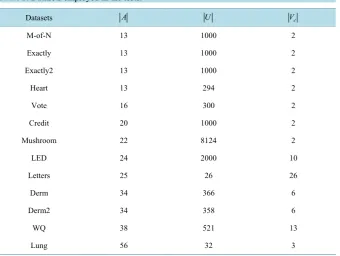
Table 5 denotes by A the cardinality of the conditional attribute set, by U the number of elements for each dataset and by Vd the number of classes of the dataset.

All these datasets were downloaded from the UCI Machine Learning Repository [22]. The 5720 tests were executed in a PC with a quadcore 3.4 GHz processor and 16 GB of main memory. All metaheuristics were coded in Perl (Practical Extraction and Report Language) using object-oriented programming. The datasets were stored in the Database Management System (DBMS). Perl is suitable for the proposed application, since it is 1) an interpreted language, 2) it is portable, 3) deals easily with strings, and 4) provides text manipulation and pattern matching. DBMS makes easy the storing and retrieval of data and provides evaluation functions in the SQL (Structured Query language).

The benchmarks results, taken as a reference, are those found in [5] and [15]. These results refer to the use of the metaheuristics ACO, SA, GA and TS to perform the calculation of reducts in RST aiming at classification for the set of databases described inTable 5. These results were obtained employing only the degree of depen-dency (γ) as evaluation function.

[image:11.595.131.472.465.721.2]

The new results obtained by the application of the proposed metaheuristics to these databases are shown in the following tables, except for VND, shown in a table that summarizes the results, for convenience. VND seems more suitable to be used as a local search scheme, as discussed in [21]. However, VND is also employed as a local search scheme instead of the standard local search scheme. It is worth to note that both VNS and DCS were evaluated using as local search scheme either standard one or VND itself. In addition, VNS and DCS were

Table 5. Datasets employed in the tests.

Datasets A U Vd

M-of-N 13 1000 2

Exactly 13 1000 2

Exactly2 13 1000 2

Heart 13 294 2

Vote 16 300 2

Credit 20 1000 2

Mushroom 22 8124 2

LED 24 2000 10

Letters 25 26 26

Derm 34 366 6

Derm2 34 358 6

WQ 38 521 13

(12)

[image:12.595.129.467.170.444.2] [image:12.595.127.469.481.723.2]

also evaluated using different evaluation functions: RSAR (γ function) or Relative Dependency (κ function). Table 6show results for VNS, and Table 7, for DCS. Each entry of the table denotes the reducts as Q(n)_, where Q denotes the cardinality and the superscript n denotes the number of times a reduct with such cardinality was obtained, out of the 20 executions of the given metaheuristics. This superscript was omitted when n = 20, i.e.

Table 6. Reducts obtained by the VNS metaheuristics using either the standard or the VND local search schemes for the 13 considered datasets.

Datasets A VNS(γ)-s VNS(κ)-s VNS(γ)-v VNS(κ)-v

M-of-N 13 6 6 6 6

Exactly 13 6 6 6 6

Exactly2 13 10 10 10 10

Heart 13 6 6 6 6

Vote 16 8 8 8 8

Credit 20 _L88 8 8 8

Mushroom 22 3 _L83 3 3

LED 24 5 5 5 5

Letters 25 8 8 8 8

Derm 34 6 6 6 6

Derm2 34 8(9)_L169(11) 8(18)_L169(8) 8(17)_L169(3) 8(12)_L169(8)

WQ 38 12(15)_L1613(5) 12(16)_L813(4) 12(19)_L1613(1) 12(19)_L1613(1)

Lung 56 3(19)_L164(1) _L163 _L163 _L83

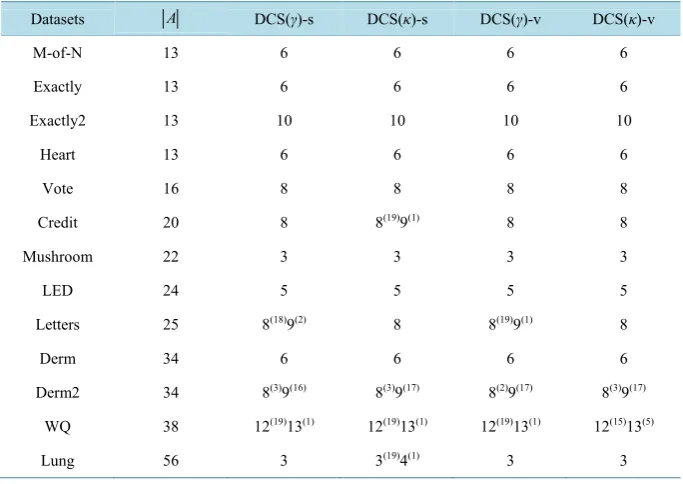
Table 7. Reducts obtained by the DCS metaheuristics using either the standard or the VND local search schemes for the 13 considered datasets.

Datasets A DCS(γ)-s DCS(κ)-s DCS(γ)-v DCS(κ)-v

M-of-N 13 6 6 6 6

Exactly 13 6 6 6 6

Exactly2 13 10 10 10 10

Heart 13 6 6 6 6

Vote 16 8 8 8 8

Credit 20 8 8(19)₉(1) ₈ ₈

Mushroom 22 3 3 3 3

LED 24 5 5 5 5

Letters 25 8(18)₉(2) ₈ ₈(19)₉(1) ₈

Derm 34 6 6 6 6

Derm2 34 8(3)₉(16) ₈(3)₉(17) ₈(2)₉(17) ₈(3)₉(17)

WQ 38 12(19)₁₃(1) ₁₂(19)₁₃(1) ₁₂(19)₁₃(1) ₁₂(15)₁₃(5)

(13)

the same cardinality Q was obtained for all executions. In the case of VNS, most of the results were obtained with the lower Hamming distance L = 4. However, for test cases where higher values of L yielded better results, the value of L (8 or 16) appeared below the resulting cardinalities. As mentioned in Section 4.1, the default val-ue for standard local search is L = 1, and for the VND local search scheme is L = 2.

It can be observed that VNS yielded better reducts using VND that the standard local search scheme. VNS results are in general slightly better than those of DCS. A comprehensive comparison is given byTable 8 that depicts an average ranking of the results for all databases using a skill score described below. The same table also ranks average processing times for all databases, showing that DCS is in general faster. These processing times are presented inTable 9for all the variants of the metaheuristics.

[image:13.595.129.467.263.718.2]

In face of the multitude of reducts obtained by the different metaheuristic variants for the 13 datasets, it is dif-ficult to compare the performance of the different metaheuristics. Therefore, a new metric was introduced,

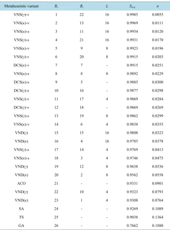
Table 8. Ranking of the average skill score (Rs), ranking of the average processing time (Rt), VNS hamming distance (L), average skill score (Savg) and standard deviation (σ) of the skill score for each proposed metaheuristic variant considering 20 executions for the 13 datasets.

Metaheuristic variant Rs Rt L Savg σ

VNS(γ)-v 1 22 16 0.9985 0.0055 VNS(κ)-v 2 13 16 0.9969 0.0111 VNS(κ)-s 3 11 16 0.9954 0.0120 VNS(γ)-s 4 21 16 0.9931 0.0170

VNS(κ)-v 5 9 8 0.9923 0.0196

VNS(γ)-v 6 20 8 0.9915 0.0203

DCS(κ)-v 7 7 - 0.9915 0.0251

VNS(κ)-s 8 8 8 0.9892 0.0229

DCS(κ)-s 9 5 - 0.9885 0.0300

DCS(γ)-s 10 16 - 0.9877 0.0298 VNS(γ)-v 11 17 4 0.9869 0.0284 DCS(γ)-v 12 18 - 0.9869 0.0269 VNS(γ)-s 13 19 8 0.9862 0.0299

VNS(κ)-v 14 6 4 0.9838 0.0355

VND(γ) 15 15 16 0.9808 0.0323

VND(κ) 16 4 16 0.9785 0.0378

VNS(γ)-s 17 14 4 0.9769 0.0413

VNS(κ)-s 18 3 4 0.9746 0.0475

VND(γ) 19 12 8 0.9638 0.0536

VND(κ) 20 2 8 0.9562 0.0558

ACO 21 - - 0.9331 0.0901

VND(γ) 22 10 4 0.9323 0.0793

VND(κ) 23 1 4 0.9308 0.0764

SA 24 - - 0.9269 0.1089

TS 25 - - 0.9038 0.1364

(14)

[image:14.595.128.467.110.321.2]

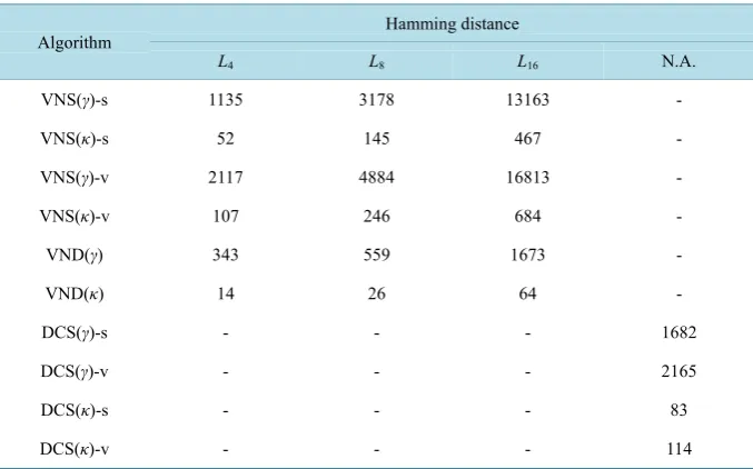
Table 9. Average execution times (in seconds) for 20 executions for each one of the 13 da-tasets.

Algorithm Hamming distance

L4 L8 L16 N.A.

VNS(γ)-s 1135 3178 13163 -

VNS(κ)-s 52 145 467 -

VNS(γ)-v 2117 4884 16813 -

VNS(κ)-v 107 246 684 -

VND(γ) 343 559 1673 -

VND(κ) 14 26 64 -

DCS(γ)-s - - - 1682

DCS(γ)-v - - - 2165

DCS(κ)-s - - - 83

DCS(κ)-v - - - 114

called skill score called skill score (S), as a means to evaluate the quality of the reducts. Considering a given da-taset, the skill score S for N executions of a metaheuristic is defined as follows taking into account the obtained reducts with M different cardinalities:

min 1 M

i i i Q C S

N = C

=

∑

(11)

where, Cmin is the cardinality of the best reduct found by any execution of any metaheuristic (assumed as being the minimum cardinality), Ci denotes the i-th cardinality, while Qi denotes the number of reducts obtained with such cardinality out of the N executions. Therefore, if all executions yield reducts with the minimum cardinality, the skill score will be equal to one. The summation imposes a penalty for obtaining bad reducts many times. As an example, the 20 executions of VNS(γ)-s for the Derm2 dataset inTable 6, yielded 8(9)₉(11)_{. Since 8 is the best} cardinality found, the resulting the skill score is

(

8 20

) ( ) (

×_9 8 + 11 9

)

_ or 0.9389.

Table 8presents the average skill score (and its mean deviation) of each metaheuristic variant for a particular choice of parameters (local search scheme, evaluation function and L). Considering a particular metaheuristic variant, it is executed 20 times for each of the 13 datasets, yielding the corresponding 13 partial averages. The average skill score is then given by the average of these partial averages. A compilation of such results sepa-rately for each dataset would be too extensive. Each choice of metaheuristic variant parameters is then ranked in the table according its skill score. It is worth to note that all the proposed metaheuristics variants attained better skill scores, in average, than the ones proposed in [5]. Observing the results for each dataset, the proposed me-taheuristic variants always found reducts with minimum cardinality. For a given dataset, such minimum is not necessarily the best minimum, but the better minimum found in the tests (i.e. not an optimal minimum, but more likely a suboptimal minimum). However, some few sets of executions of ACO or TS may have yielded better reducts for some datasets than some proposed metaheuristic variants. For instance, for the dataset Letters, ACO obtained 20 times reducts with cardinality 8 (not shown here). The variants of the proposed metaheuristic VNS, VND and DCS achieved the same result, except for VND (γ) with L = 8 and DCS (κ)-s that obtained 8(19)₉(1)_and for DCS (γ)-s that obtained 8(18)₉(2)_{, but these can also be considered good solutions.}

The choice of the evaluation function, RSAR (γ) or Relative Dependency (κ), does not seem to make differ-ence in the cardinality of the reducts for the proposed metaheuristic variant. However, as explained ahead, the use of Relative Dependency implies in a much lower processing time. On the other hand, for VNS and VND va-riants, the use of higher values of L tends only to improve slightly the quality of the reducts for some databases. Typically L = 4 ensures good reducts, while L = 8 or L = 16 may allow better reducts for some few datasets.

(15)

there is a trade-off between the quality of the results and processing time. Unfortunately, [5] or [15] did not mention execution times for ACO, SA, GA or TS, concerning the calculation of reducts for cited datasets. However, some conclusions can be drawn for the proposed metaheuristic variants based on their average total processing times, as shown inTable 9. Each entry corresponds to the average execution time for a particular va-riant, i.e. the average of the 20 executions for each one of the 13 datasets. In the case of VNS and VND, average times appear for the different Hamming distances.

A first point about computational performance is that the proposed metaheuristic and heuristic variants ex-ecutes much faster (in general) using the Relative Dependency as evaluation function. On the other hand, the results obtained for ACO, SA, GA and TS were obtained using only the RSAR evaluation function. A second point is the choice of local search scheme in VNS and DCS variants. The choice of VND as local search scheme demands a slightly higher processing time, as would be expected, since the standard local search is simpler. A third point is the cardinality of the neighborhood structure (L). The choice of L = 4 seems suitable, since L = 8 or L = 16 roughly doubles or triplicates processing times, respectively. This issue does not apply for DCS variants.

The following discussion assumes the use of Relative Dependency evaluation function. In general, VNS va-riants obtained the best reducts, but using more process time. The average skill scores of VNS vava-riants with L = 16 are the top ranked inTable 8, but it can be considered acceptable choices the use of VNS with L = 8 (up to 30 seconds using standard local search or up to 50 seconds using VND local search) or even VNS with L = 4 (up to 10 seconds using standard local search and up to 20 seconds using VND local search).The variants of VND are much faster due to its simplicity, demanding less than one second with L = 4 or L = 8 for most databases, but with lower ranked skill scores. Finally, DCS attained better skill scores than VND variants (except for the Mu-shroom dataset), but with processing times similar to VNS variants with L = 8. DCS variants demand a higher limit number of iterations to converge (30 iterations) than VNS variants, which require 10 iterations.

In particular, DCS variants obtained the best reducts only for the Lung dataset (cardinality 3), in comparison to most of the results of VNS and VND variants, that obtained reducts with cardinality 3 mixed with reducts with higher cardinality (4, 5 or 6). It can be noted that the best cardinality obtained by GA, ACO, SA or TS for the Lung dataset was 4. However, the computational performance of DCS variants was better than VNS or VND ones, since, in terms of skill score, the best ranked was DCS (κ)-v (7th with s = 0.9915) that had an overall av-erage execution time ranking of also 7th (corresponding to 114 seconds), while VNS(κ)-v with L = 8 (5th with s = 0.9923) has a corresponding average time ranked at 9th (corresponding to 246 seconds).

In general, VNS variants always converge to an optimal or suboptimal reduct. The top six skill scores in Ta-ble 8 were obtained by VNS variants using either of the local search schemes or either of the evaluation func-tions. Variants that employ the Relative Dependency evaluation function (κ) are much faster.

6. Final Remarks

This work presented the innovative application of three metaheuristics for attribute reduction based on the Rough Set theory (RST). Subsets of attributes/features called reducts are obtained for the given dataset and al-low performing classification using the same dataset with reduced dimensionality. Normally, classification and computational performance are improved. Large and complex datasets require that the reduct calculation in RST be formulated as an optimization problem, and therefore solved by some metaheuristic. A standard metaheuris-tics for this purpose is GA, but others were proposed in the late years, like ACO, SA, or TS. Some commonly employed datasets were adopted to test these metaheuristics.

Variants of the three proposed metaheuristics, VNS, VND and DCS, were extensively tested for attribute re-duction in RST with a set of well known datasets. In particular, DCS is a new metaheuristics developed for this work. The proposed metaheuristic variants obtained reducts with equal or better (i.e. lower) cardinality than GA, ACO, SA or TS, except for VND. VNS and DCS can probably be employed in a competitive manner for reduct calculation in RST at a (probably) lower computational cost, in part due to the choice of a less costly evaluation function. VND is a deterministic algorithm, while VNS and DCS have some stochasticity, but are inspired in deterministic methods. This would explain the fast convergence they present: the limit number of iterations was 10 for all variants of VNS, and 30 for the DCS ones.

(16)

algo-rithm and that, sometimes, can be optimized only for a particular dataset, with loss of generality and at cost of many executions.

It would be difficult to choose the best metaheuristic variant between VNS and DCS. Results show that VNS variants have more robustness, i.e. always find good reducts, but at the cost of higher processing time. In general, due to its deterministic nature, VND variants demanded far less processing time, but generated reducts slightly poorer than VNS variants. It is worthy to note that VND variants did not seem prone to get trapped in local mi-nima of the search space. The better choice may be guided by the dimensionality of the dataset: considering the same number of elements, a dataset with low dimensionality would be tackled with better accuracy by VNS, while another with high dimensionality, by DCS, since VNS would require too much processing time.

Finally, the new metaheuristic proposed in this work, DCS is a VNS variation that adopts a more aggressive search scheme, only accepting neighbor solutions with lower cardinality. DCS variants were competitive com-pared to VNS and VND variants, and for some datasets, obtained the best reducts (i.e. reducts with lower cardi-nality). Processing times of DCS variants are higher than those of VND variants, but lower than processing times of VNS variants with medium/high cardinality of neighborhood structure. Therefore, DCS variants seem to provide a good trade-off between the quality of the results and processing time.

The alternative metaheuristics proposed in this work applied for reducts calculation in RST performed better than formerly employed metaheuristics for the considered datasets, achieving the 20 top positions in the ranking of average skill scores. The three alternative metaheuristics (VNS, VND and DCS) do not require the tuning of specific parameters having thus more robustness than these previous approaches. In particular, DCS provides competitive results with lower processing time.

In recent years, a myriad of new optimization algorithms have been proposed for many different areas. A fur-ther work would exploit such new algorithms in the scope of attribute reduction in RST in order to tackle data-bases with even higher dimensionality than those presented here.

Acknowledgements

Authors Alex SandroAguiar Pessoa and Stephan Stephany are thankful to the Brazilian Council for Scientific and Technological Development (CNPq) for grants 140161/2010-4 and 305639/2012-9, respectively.

References

[1] Pawlak, Z. (1982) Rough Sets. International Journal of Computing and Information Sciences, 11, 341-356. http://www.springerlink.com/index/r5556398717921x5.pdf

[2] Komorowski, J., Pawlak, Z., Polkowski, L. and Skowron, A. (1999) Rough Sets: A Tutorial. Warsaw. http://secs.ceas.uc.edu/~mazlack/dbm.w2011/Komorowski.RoughSets.tutor.pdf

[3] Ohrn, A. (1999) Discernibility and Rough Sets in Medicine: Tools and Applications. Norwegian University of Science and Technology, Trondheim.

[4] Jensen, R. and Shen, Q. (2003) Finding Rough Set Reducts with Ant Colony Optimization. Proceedings of the 2003 UK Workshop on Computational Intelligence, 15-22. http://users.aber.ac.uk/rkj/pubs/papers/antRoughSets.pdf

[5] Hedar, A.-R., Wang, J. and Fukushima, M. (2008) Tabu Search for Attribute Reduction in Rough Set Theory. Soft Computing, 12, 909-918. http://www.springerlink.com/index/c4181mh5l23816u3.pdf

[6] Pessoa, A.S.A., Stephany, S. (2012) Feature Selection with New Metaheuristics in the Rough Sets Theory. XXXIV Na-tional Congress of ComputaNa-tional and Applied Mathematics, 1, 1-7.

[7] Hansen, P. and Mladenovic, N. (2003) A Tutorial on Variable Neighborhood Search. Montreal. http://yalma.fime.uanl.mx/~roger/work/teaching/mecbs5122/5-VNS/VNS-tutorial-G-2003-46.pdf

[8] Han, J., Sanchez, R. and Hu, X. (2005) Feature Selection Based on Relative Attribute Dependency: An Experimental Study. Rough Sets, Fuzzy Sets, Data Mining, and Granular Computing, 3641, 214-223.

http://www.springerlink.com/index/743agvmf3etlaq0p.pdf http://dx.doi.org/10.1007/11548669_23 [9] Zadeh, L.A. (1965) Fuzzy Sets. Information and Control, 8, 338-353.

http://dx.doi.org/10.1016/S0019-9958(65)90241-X

[10] Shafer, G. (1976) A Mathemathical Theory of Evidence. Princeton University Press, Princeton.

[11] Dempster, A.P. (1967) Upper and Lower Probabilities Induced by a Multivalued Mapping. The Annals of Mathemati-cal Statistics, 38, 325-339. http://dx.doi.org/10.1214/aoms/1177698950

(17)

http://dx.doi.org/10.1016/S0165-0114(99)80004-9

[13] Nicoletti, M. do C. and Uchôa, J.Q. (1997) Rough Sets under the Perspective of Pertinence Function. 3rd Brazilian Symposium on Intelligent Automation, Vitoria, Brazil, 307-313, in Portuguese.

[14] Chouchoulas, A. and Shen, Q. (2001) Rough Set-Aided Keyword Reduction for Text Categorization. Applied Artificial Intelligence, 15, 843-873. http://www.tandfonline.com/doi/abs/10.1080/088395101753210773

[15] Jensen, R. and Shen, Q. (2005) Semantics-Preserving Dimensionality Reduction: Rough and Fuzzy-Rough-Based Ap-proaches. IEEE Transactions on Knowledge and Data Engineering,16, 1457-1471.

http://ieeexplore.ieee.org/xpls/abs_all.jsp?arnumber=1350758

[16] Holland, J.H. (1975) Adaptation in Natural and Artificial Systems. University of Michigan Press, Ann Arbor. http://www.citeulike.org/group/664/article/400721

[17] Goldberg, D.E. (1989) Genetic Algorithms in Search, Optimization, and Machine Learning. Addison-Wesley, Boston. http://www.mendeley.com/research/genetic-algorithms-in-search-optimization-and-machine-learning/

[18] Kirkpatrick, S., Gelatt, C.D. and Vecchi, M.P. (1983) Optimization by Simulated Annealing. Science,220, 671-680. http://www.sciencemag.org/content/220/4598/671.shorthttp://dx.doi.org/10.1126/science.220.4598.671

[19] Glover, F. and McMillan, C. (1986) The General Employee Scheduling Problem. An Integration of MS and AI. Com-puters Operations Research, 13, 563-573. http://dx.doi.org/10.1016/0305-0548(86)90050-X

[20] Colorni, A., Dorigo, M. and Maniezzo, V. (1991) Distributed Optimization by Ant Colonies. European Conference on Artificial Life,Paris, France 134-142.

[21] Hansen, P. and Mladenovic, N. (1997) Variable Neighborhood Search. Computers & Operations Research, 24, 1097- 1100. http://www.sciencedirect.com/science/article/pii/S0305054897000312

http://dx.doi.org/10.1016/S0305-0548(97)00031-2

[22] Blake, C.L. and Merz, C.J. (1998) UCI Repository of Machine Learning Databases. University of California, Oakland.

(18)