Equalisation and Fiscal Competition

Munich Personal RePEc Archive

Equalisation and Fiscal Competition

Rizzo, Leonzio

May 2000

Online at

https://mpra.ub.uni-muenchen.de/5335/

Università degli Studi di Ferrara

DIPARTIMENTO DI ECONOMIA, ISTITUZIONI, TERRITORIO

Corso Ercole I D'Este n.44, 44100 Ferrara

Quaderni del Dipartimento

n.7/2000

May 2000

Equalization and Fiscal Competition

May 2000

Equalization and Fiscal Competition

Leonzio Rizzo

Università degli Studi di Ferrara STICERD-London School of Economics

Abstract

The paper’s aim is to link two different issues: equalization and fiscal competition. In the model there are two regions: the first one has rich citizens and the other one has poor citizens. Regional representatives in a federal Council must decide on the introduction of an equalization transfer based on fiscal capacity. Regions choose tax rates on a consumption good and the citizens choose where to buy the consumption good. We show that the existence of the transfer stimulates regions to choose higher tax rates. The economic insight for this result is that the existence of a mobile tax base generates a negative fiscal externality on each regional planner. We show that the equalization transfer presents a wider range of agreement opportunities between regional representatives to correct the inefficient levels of tax rates than a compensation transfer does. This is because efficiency gains are equalized with the introduction of an equalization transfer

JEL classification: H21, H23.

Keywords: fiscal competition, equalization, transfer, externality, tax-rate.

0. Introduction

Fiscal decentralization is normally justified by two factors. Firstly, local taxes reflect citizens' preferences much more than central taxes. Secondly, the management of local public expenditure would be more efficient than it would be if taxes were centralized.

However, in a Federation the geographical subset, where regional Government taxes, can not coincide with the subset where the tax-base of the residents of each region is distributed. In this case with free mobility of persons, goods and capital each region fixes its tax rate without taking into account the benefits in revenue and/or social welfare to the other regions (Mintz and Tulkens 1986; Wilson, 1991; Wildasin, 1988, 1991). That generates fiscal externalities. The extent and direction of these externalities depends on the interaction of two effects: public consumption effect and private consumption effect. The first effect is due to the region raising its tax-rate, which, if its tax-base is mobile, will benefit the other regions in revenue terms: in this way the region will fix a too-low tax-rate from a federal point of view. The second effect comes out only if the region is exporting the taxed good. In this case the region does not take into account that the good is also consumed by the citizens of the other regions and will fix a too-high tax-rate from a federal point of view.

In the EC fiscal competition is a concrete issue if we think of taxes like VAT or excises on fuel and alcohol. With taxation not co-ordinated the risk of cross-border shopping becomes real. In the 80’s we experienced cases of cross-border shopping: Denmark-Germany and Ireland-United Kingdom (Fitzgerald et alii 1988, 1995). In ‘84 Ireland was forced to lower taxes on whiskey and TV because of the huge cross-border shopping of its residents in Northern Ireland. Cross-border shopping is also recently becoming a problem for the United Kingdom with Europe for products like wine and beer which are taxed vmuch more in UK than in the continental states (Crawford, Tanner, 1995).

According to the above mentioned empirical studies, that fiscal competition stimulates regions to lower equilibrium tax-rates, has a theoretical explanation: regions in their objective function give high weight to the collected revenue and the public consumption effect prevails.

Normally States or regions make some co-operative agreements to define tax-bases or tax-rates or to share taxes with the federal government. In this latter case the way that the federal revenue is given back can be crucial to the extent of fiscal externalities or the fairness level in the public good provision among different regions.

these transfers reducing the higher revenue that regions get by attracting tax-base and by compensating other regions, which are losing tax-tax-base. It is the case when the equalization transfer can transfer back a quota of the migrated tax-base.

Empirical literature (Bird and Slack, 1990; Bird, 1993) on equalization transfer does not take into account the influence in the introduction of equalization transfers on the fiscal decisions of the regions. In our work we try to study these effects in a framework with asymmetric per-capita tax-bases and with revenue maximiser regions.

We study the determinants of unanimous agreements on the introduction of an equalization system by the regions. In a context, where a federating process is starting up, as in the European Community or Italy, this issue is crucial. Can the equalization system come out of an agreement among the members of the Federal State?

We can think of an institutional framework like the one of the European Community where the Commission could propose the structure of the equalization system, but after the Council should approve it. We explore the possibility linked to the difference in per-capita tax-base that the choice of the federal Council brings a Pareto improvement in the level of the federal collected revenue. We show how an equalization transfer has greater possibilities to be introduced with the consensus of both regions than a compensation transfer does, given that both transfers introduce some kind of inefficiency in the revenue collection.

The paper is organised as follows. In the first section we describe the model . In the second section we explain and comment on the solution of the model. We explore the possible equilibria with equalization. In the third section we consider the possibility that the federal Council chooses a compensation transfer and we compare the two transfers.

1. Description of the model

There are two regions, 1 and 2. In each region there are n consumers uniformly distributed.

There are two firms, one in each region, with identical constant return to scale technology, which uses labour as input. Each firm produces the same homogeneous consumption good y. Production prices in this case are fixed.

region 2. These are goods for which it is difficult to find substitutes so if people are used to consume a certain quantity they will not change their demand much even if prices change. We take account of this characteristic of the good by making the simplifying assumption that demands are rigid with respect to the prices. The reservation prices of the consumers of the two regions are such that the new tax-rate equilibrium, after the introduction of the transfer, will not induce a change in demand with respect to the no-equalization case. From now on we will refer to region 1 as the poor region and region 2 as the rich region.

In each region there is a leviathan government which maximises its revenue by choosing tax on the consumption good y. This assumption on the objective function will cause a public consumption effect which will stimulate too-low Nash equilibrium tax-rates with respect to the federal optimal solution (Mintz, Tulkens, 1986).

A Council composed of the representatives of the regions decides on the introduction of an equalization transfer based on difference between per-capita tax-bases. The decisions of the Council are taken at unanimity. This is the same rule of the EC Council when it has to approve fiscal acts. So the Council accepts to introduce the equalization transfer if it is Pareto-improving.

At the first stage, the Council, composed of the representatives of the two regions, decides on the introduction of an equalization transfer.

The introduction of the equalization transfer is likely to stimulate moral hazard problems in both regions. The transfer assures the poor region that it will receive a revenue quota from the other region, which can stimulate the poor region to decrease its effort in the control and development of its tax-base. The rich region will also have less incentive to control its tax-base because a quota of its revenue will go to the other region. Another example can be that when the states have to inform a federal organism with data about their tax-base. The states have incentives to provide biased information to get (give) the highest (lowest) amount of revenue. This can behaviour can induce the states to expect a loss in revenue after the introduction of the transfer.

We do not model the asymmetric information problem (Bordignon et alii, 1996), but we take account of the consequences on the collected revenues of the behaviour of the regional governments. We make the assumption that the introduction of an equalization transfer stimulates a loss in revenue which is a linear positive function of the equalization level α. The higher the level of the transfer is, the higher the disincentive to control the tax-base or the higher the risk to lose revenue because the other states are providing false information.

At the third stage each consumer decides where to buy the good knowing that crossing the border implies a cost δ per unit of distance from the border.

2. The model

The model is solved by backwards induction. At the third stage we determine tax-base flow from one region to another. At the second stage regions choose tax-rates by maximising tax-bases. At the first stage, once we have the equilibrium tax-rates we can calculate equilibrium revenues. The representatives of the regions choose whether to introduce or not the transfer by comparing the revenue functions they would have with the transfer with those without the transfer.

2.1 The third stage

Take region 2. Two conditions must be satisfied for the consumer of region 2 to cross the border and buy the good in region 1. The first one is that the surplus the consumer obtains by buying the same quantity she is ready to buy in her region is higher than the surplus the same consumer would get in her region:

Insert fig. 1

(1) r2y2 −s1y2 −δd >r2y2 −s2y2 ⇔

−

>

s s

y d

2 1

2

The second condition asks for non-negative surplus:

(2) r₂y₂ −s₁y₂ −δd >0.

1

r, r₂ reservation price net of production cost, in region 1 and 2, at which the consumer is indifferent between buying ymor ym −1 units of the good

where m=1,2;

δtransport cost per unit of distance to the border;

d distance from the border of the consumer indifferent as to whether he is to buy in region 1 or in region 2. As consumers are uniformly distributed d

indicates also the consumers’ quota going from region 2 to region 1.

s₁ and are per-unit tax of the two regions on the good s₂ y.

2.2 Second stage

The total demand function of good y of each region for a given tax-rate of the other region is:

B

n y s s y s

n s s y s

1

1

2 1

2 2 1

1 2

1 2 1

1

=

+ − 



 _ ≥

− − 



 



 ≤

δ

δ

se s (3a)

B

n y s s y s s

n s s y s s

2

2

1 2

1 1 2

2 1

1 2

1

=

+ − 



 



 ≥

− − 



 



 ≤

δ

δ

se (4a)

se (4b)

2

Total consumption demands are very similar to the ones of the Kanbur and Keen model. If in our model we substitute the demand value with the size value of the regions (in the Kanbur and Keen model regions differ for their size) and vice versa for the size we fall into the Kanbur and Keen case. Total regional tax-bases are still the same, but per-capita regional tax-bases differ from our model: they are the same in both regions in the Kanbur and Keen model.

2.2.1 An equalization transfer

The solution of the following equation:

α B α

n tr

B B n

2 2

1 2

2

+ = +

gives:

tr B n

B n

2

1 2

1 2

= _ −    α

where:

B1 tax-base of region 1

B₂ tax-base of region 2

α equalization rate

tr2 is the transfer that region 2 will receive or give to equalize a quota α of

per-capita tax-bases.

Symmetrically one can obtain tr1. The total equalization transfer from

one region to the other is:1

(5) TR B n

B n

p = ± −

 

 

  α 1

2

1 2

If we substitute in (5) (3a) and (4b), or (3b) and (4a) we get the expression for the transfer from one region to the other which equalizes per-capita revenue at the equalization rate α:

(6)

(

)

(

)

TR

n y y s s y s s

n y y s s y s s

p =

±  − + −





 ≤

±  − + −



  ≥ 

  

  

α

δ

α

δ

1 2 1 2

1 2

2 1

2 1 2

1 2

2 1

1 1 2

(a)

(b)

Take the case s₁ ≤s₂. The transfer is composed of two terms. The first

one, ±αn 1

(

y −y

)

With open frontiers and s₁ <s₂, there is a consumers’ quota going from region 2 to region 1. This phenomenon makes the rich region have a lower tax-base than it would have in the autarkic case. The reverse is true for the

poor region. In fact in (6a) we have the term ±α −

δ

n s2 s1 y2, which is

positive for the rich region and negative for the poor one. This term is the transfer to the rich region of a α-quota of the tax-base migrated to the poor region.

In the Kanbur and Keen model the only reason for the difference in the equilibrium tax-bases is cross-border shopping. In their model, where per-capita tax-bases are the same, the equalization transfer is:

TR

s s

n s s

s s

n s s

p =

± − ≤

± − ≥



  

  

α δ

α _δ

2 1

1 2

2 1

1 2

2

1

where:

n1 consumers of region 1

n2 consumers of region 2

2.2.2 Best reply functions and the equilibrium

The introduction of an equalizing can cause a loss in revenue. We discussed the reasons of this loss in section 1. We express the loss as a linear function of the equalization rate:

κα.

The higher κ is, the higher the loss for each level of α is. Thus κ measures the level of inefficiency due to the existence of the transfer.

(7)

(

)

(

)

       ≤     _{− −} − +       ₊ − ≥     _{− −} − +       ₊ − = 1 2 1 1 2 1 2 1 1 2 1 1 1 2 2 1 2 1 2 2 1 2 1 1 1 -2 1 -2 1 s s y s s y y n y s s y n s s s y s s y y n y s s y n s R p κα δ α δ κα δ α δ (8)

(

)

(

)

       ≤     _{− +} − +       ₋ − ≥     _{− +} − +       ₋ − = 1 2 1 1 2 2 1 1 1 2 2 2 1 2 2 1 2 2 1 2 1 2 2 2 2 -2 1 -2 1 s s y s s y y n y s s y n s s s y s s y y n y s s y n s R _p κα δ α δ κα δ α δ

region 1 maximises (7) with respect to s1 and region 2 maximises (8) with

(9)

(

)

(

)

s s s s s 1 2 2 2 2 1 2 1 2 = + + ≤ + + + ≥      

δ α δ λ α

δλ α δ λ α

+ (10)

(

)

s s s s s s s 2 1 1 1 1 1 1 1 2 1 2 = + + ≤ + + ≤ ≤ + + +    _ ≥ +          

δ α δ α

δ α δ_λ α

δ λ α δ λ α

where: λ = y ≤

y

1

2

1

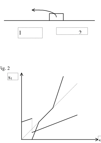
Insert fig.2

In (9) we see how region 1, that has a lower per-capita tax-base, chooses a tax-rate higher than the one of region 2 for very low s₂ levels. Region 2’s tax-rate is so low that it is not worth it for region 1 to lower its tax-rate in order not to allow its residents to migrate. If region 2’s tax-rate rises, region 1 raises its tax-rate of one half. Its tax-rate will stay in the regime

s₁ >s₂ until some s₁ level. This level is lower the higher the difference in per-capita tax-bases is and the lower transport cost is. At this s1 level a marginal

shopping direction. The higher the per-capita tax-base difference between the two regions, the lower region 2’s tax-base with respect to region 1’s tax-base and of course the lower the s1 level at which region 2 undercuts.

In (10) where we consider the best reply function of region 2, the region raises its tax-rate, when the other region will raise its too, without ever undercutting. Difference in per-capita tax-base never makes a jump in the best reply function worth it.

If we combine (9) and (10) we can state the following proposition:

Proposition 1: If λ ≤1 and min

[ ]

r₁,r₂ ≥δ +α then a unique Nash equilibrium exists in pure strategies:

s₁ 1

3 2 3

* =  +



 

 +

δ λ α

s₂ 2

3 1 3

* =  +



 

 +

δ λ α

Proof: see appendix A2.

The poor region chooses a lower tax-rate than the one the rich region chooses. s₁ =s₂ cannot in fact be an equilibrium because region 1’s tax-base elasticity is lower than region 2’s. Suppose that s2 is the equilibrium tax-rate

rate the base migrating to region 1 is higher than the migration of tax-base from 1 to 2, given 2’s tax-rate. Indeed decrease of s1 leads to a rise in the

revenue of region 1. This is the reason why Nash equilibrium tax-rates are such that s₁ <s₂. This result is due to Kanbur and Keen (1993). In their model the asymmetry in population size of the two regions determines the difference in the elasticity of the total tax-bases we have illustrated. Even if we have an asymmetry in the level of per-capita consumption, as in our case, the total tax-bases are the same as the ones of the Kanbur and Keen model if we exchange per-capita consumption with size. That explains why our model replicates the Kanbur and Keen result. What is important is the asymmetry in the total tax-bases.

2.3 The equalization effect on the fiscal externality

What is new in the model is the introduction of an equalization transfer stimulates higher tax rates. The regional planner raises its tax-rate because the equalization transfer is composed of a part implying a limitation of the effect of mobility. A quota of the mobile tax-base will “come back”. The regional planner will take this part into account in choosing tax-rates.

To better understand what happens let us examine the first order conditions of the federal government whose welfare function is:

) , ( ) ,

( _{1 2 2 1 2}

1 s s R s s

R

and evaluate them at the Nash equilibrium:

(11)

( )

, 0

* 2 2 1 * 2 * 1 2 1 ≥ = ∂ ∂ = ∂ ∂ δ s y s s s R s W

(12)

( )

, 0

* 1 2 2 * 2 * 1 1 2 ≥ = ∂ ∂ = ∂ ∂ δ s y s s s R s W

Each region does not take into account that a raise in its tax rate, given the tax rate of the other, will benefit the other region, so tax rates are lower than the efficient ones are. (11) and (12) are exactly the analytical expressions of the fiscal externalities.

The first order conditions related to the Nash equilibrium are the following (s₁* ≤s₂*):

(13) 2 2 0

1 2 2 1 1 1

1 − + =

     ₊ − = ∂ ∂ δ α δ δ y y s y s s y s R

(14) 2 2 0

2 2 1 2 2 2

2 − + =

     ₋ − = ∂ ∂ δ α δ δ y y s y s s y s R

In (13) the fiscal externality effect on the decision of Region 1 is given

by δ 2 1 y s

− , which in equilibriun is exactly the value, with opposit sign, we

have found in (11). The equalizing transfer effect is given by

δ α y2

. This

region, will benefit the other region, because it will get this benefit through the equalizing mechanism.

2.4 Some descriptive evidence

It is interesting to compare two federal countries like Canada and Australia with two different distribution of taxing power.

If we look in the Statistics on tax revenues (OECD, 1996) at the item taxes on production and sales (which essentially includes sales taxes, VAT taxes and excises taxes) we can observe the following:

Percentage collected at State/Provincial level Canada 51

Australia 14

which tells us that Canada has a much more decentralized taxing power than Australia. According to the theory we would expect Australia to raise more revenue than Canada because Australia should have lower fiscal externalities, but if we look at the tax revenue of the federation, relative to production and sales, as percentage of total tax revenue of the federation, we get:

In this result general taxes (sales and VAT taxes) are determinant.

Even if in Canada taxes on production and sales are much more decentralised, Canada is able to raise a higher quota of total revenue than Australia does.

This can be due to agreements among provinces. But it is not easy to reach them: only recently Newfoundland, Nova Scotia and NewBrunswick reached an agreement on a harmonised sales tax (1997). The other provinces still autonomously decide their retail sales tax.

The low harmful impact of fiscal competition could be explained by the existence of a transparent equalizing system based on differences on tax-bases, like the Canadian system, which is very similar to the transfer we adopted in the model. In Canada the transfer is calculated for 33 types of taxes. (some of them are: sales taxes, taxes on tobacco, wine, beer, fuel).

2.5 First stage

At the first stage the federal Council decides whether to introduce or not the transfer at unanimity. So given the absence of an equalization transfer we want to explore the determinants of the possibility of introducing an equalization transfer which Pareto-improves the revenue of the Federation.

2.5.1 The equalization transfer

(15) δ λ α

(

λ

)

−κα         + +       + = 1 2 1 3 2 3 1 2 2

1 y n

R_p

(16) δ λ α

(

λ

)

−κα

        + +       + = 1 2 1 3 1 3 2 2 2

2 y n

R _p

If we subtract from (15) and (16) the revenue raised by the regions without

the equalizing transfer, we obtain 

  



 + _−κ α

2

2

1 y

y

. Region 1 and 2 with the

introduction of the equalising system gain 2

2

1 y

y +

α and lose κα. Both

regions have the same efficiency gain because of equalization.

Both regions will not agree on the introduction of the equalization

transfer if 2 2 1 y y + ≥

κ . In this case the inefficiency due to the introduction

of the transfer is not compensated by the efficiency gain, due to the effect that the transfer have on the fiscal externalities.

3. The compensation transfer

outlined in section 1. So each region will lose revenue in the same way as before.

In our model such a compensation transfer is:

(17) TR

n s s y s s

n s s y s s

c =

± − ≤

± − ≥



  

  

β δ

β δ

2 1

2 1 2

2 1

1 1 2

d=s2 −s1 y₂

δ is the demand quota going from region 1 to region 2.

Introducing (17) limits mobility effect on the tax-rate.

We want to explore the possibility that also the introduction of the compensation transfer can Pareto-improve the Federal revenue.

If we set α=β, (17) is the second part of the equalization transfer (6). The compensation transfer is equivalent to the equalization transfer without the lump sum part.

As the equilibrium tax-rate is higher in the rich region than in the poor region, the compensation transfer is positive in the rich region and negative in the poor one.

3.1 The tax-rate incentive

The answer is yes. We noted (section 2.2.2) in the case of the equalization transfer that the term which determines the tax-rates to rise is

±α − δ

n s2 s1 y₂, which is the only term which appears in the compensating transfer.

3.2 The choice on the introduction of the transfer

After having found second stage equilibrium tax-rates which are the same as in the equalization case if substituted in the revenue functions of the two regions we get:

(18) δ λ λβ −κβ

    

  

+    

  + =

2

2 1

3 2 3 1

n y Rc

(19) δ λ β −κβ

    

  

+    

  + =

2

2 2

3 1 3 2

n y R _c

The revenue function of 1, which must give back to region 2 a part of the collected revenue, raises with β less than in the equalization case if we set

transfer the rich region takes the incentive effect on all its own tax-base. Before it transferred some of this effect to the other region.

If we subtract from (18) and (19) the revenue without the transfer we get that region 2 gains αy₂n−κα and region 1 gains αy₁n−κα from the introduction of the compensation transfer.

The reason of this difference in gain with the equalization case is that in the compensation case region 2 will not share the higher revenue it will get from the introduction of the compensation mechanism.

Region 1 in this case can be decisive in the introduction of the compensation transfer because it has a lower efficiency gain than region 2 has. This was not the case with the equalization system. Comparing the equalization levels with the compensation levels it is straightforward to state:

Proposition 2: When when κ =κ is so large that κ > y1n the compensation

transfer cannot be implemented unanimously. Moreover it can be possible

that an equalization transfer can still be implemented if κ∈

[ ]

κ,κ~ where

n y y

2 ~= 1+ 2

κ .

It is interesting to highlight that the higher the difference in tax-base, the larger the κ-range which allows the implementation of an equalizing transfer

when the regions do not agree on a compensation transfer: y y n

2 ~−κ = 2 − 1

κ .

4. Conclusions

In the paper we deal with a fiscal competition model with residents' mobility. Regions maximise their revenue by choosing tax-rates. Equilibrium tax-rates are lower than the efficient ones, because each region does not take into account that the other region can benefit in revenue terms from its decision (fiscal externality).

We analyse the determinants which drive the decision to introduce an equalization and compensation transfer.

A compensation transfer is equivalent to an equalization transfer without the redistributive component due to the difference in tax-bases. We show that it is possible to implement an equalization transfer when it is not possible to implement a compensation transfer. In both cases the introduction of the transfer induces a raise in tax-rates because of the compensation element. In the compensation case this efficiency gain is distributed proportionally to the residents’ tax base, in the equalization case the efficiency gain is equalized along the two regions. The compensation transfer could not be implemented because it could not be convenient for the region with lower tax-base. It would not gain enough to offset the costs due to the implementation of the transfer. With the equalization transfer the efficiency gain of this region will raise.

FIGURES

fig. 1

1 2

Fig. 2

s2

[image:29.595.85.294.242.536.2]

References

Bird, R. M. and Slack, E. (1990), Equalization: the Representative Tax System Revisited, Canadian Tax Journal, n. 38, pag.913-927.

Bird, R. M. (1993), Threading the Fiscal Labyrinth: Some Issues in Fiscal Decentralization, National Tax Journal, n. 46, pag.207-228.

Bordignon, M. (1995), Federalismo, perequazione e competizione fiscale,

Quaderni dell’Istituto di Economia e Finanza, n. 6, Università Cattolica, Milan.

Bordignon M., Manasse P., Tabellini G. (1996), Optimal regional redistribution under asymmetric information, mimeo, Università Cattolica, Milan.

Crawford I., Tanner, S. (1995), Alcohol Taxes and the Single European Market, IFS paper.

FitzGerald J.,Johnston J., Williams J. (1995), Indirect tax distortions in a Europe of shopkeepers, ESRI working paper, n.56, Dublin.

FitzGerald J., Quinn B., Whealan B., Williams J. (1988), An Analysis of cross border shopping, ESRI working paper n.137, Dublin.

Kanbur, R. and Keen, M. (1993), Jeux sans frontiers: tax competition and tax coordination when countries differ in size, American Economic Review, pag. 887-892.

Mintz, J. and Tulkens, H. (1986), Commodity tax competition between member states of a federation: Equilibrium and efficiency, Journal of Public Economics, n. 29, pag. 133-172.

Oates, W. E. (1972), Fiscal federalism, New York, Harcourt Brace Jovanovich.

Varian, H., R. (1992), Microeconomic Analysis, New York, Norton International Edition Student.

Wildasin, D. E. (1988), Nash equilibria in models of fiscal competition,

Wildasin, D. E. (1991), Income redistribution in a common market,

American Economic Review, pag. 757-774.

Appendix

A1 Procedure to find best reply functions

Region 1 revenue:

[

]

κα

δ α

δ _−

        _{− −} − +       ₊ − = ≥ B A B B A x t T x x x t T x t N t T 2 1

R₁ (1A)

[

]

κα

δ α

δ _−

        _{− −} − +       ₊ − = ≤ A A B A A x t T x x x t T x t N t T 2 1

R₁ (2A)

First order conditions:

(

δλ α

)

∂ ∂ _{= ⇒ = + +} 2 1 1 2 1

0 s s t

R

(3A)

(

δ α

)

∂ ∂ _{= ⇒ = + +} 2 1 2 2 1

0 s s t

R

(4A)

1st step from (3A):

(

)

(

)

α δλ α δλ α δλ α δλ + ≤ + ≥ + + + ≥ ⇒ ≥ 2 2 2 2 1 2 1 2 se if 2 1 ) 5 ( : indeed s s s s s s s s From (7A):

(

)

(

)

α δ α δ α δ α δ + ≥ + ≤ + + + ≤ ⇒ ≤ 2 2 2 2 1 2 1 2 se se 2 1 (6) : indeed s s s s s s s s 2nd step

We find revenue functions of region 1, given s₂:

      ≤     _{+ −} + ≥       _{+ + +} − = α δλ κα λ α λ α δλ κα α αδ δλ λ δ δ + -) 1 ( 2 -2 ) ( 2 2 2 2 2 1 T T Nx T T T x N R B B

substitute (6A) in (2A):

      ≥     _{+ −} + ≤       _{+ + +} − = α δ κα λ α λ α δ κα λ α αδ δλ λ δ δ + -) 1 ( 2 -2 ) ( 2 2 2 2 1 T T Nx T T T x N R B B 3rd step

We determine the best reply function on all the s2 range:

[

]

s₂ ≤minδ α δλ α+ , +

(

)

(

)

R_1p R_1p s₂ 2 s₂

2

2 2 0

# − = −α λ− −α δλ+δ λ ≥

indeed in this sub-range:

(

δλ+ +α

)

= 2 2 2 1 s s ;

[

]

(

_{) ( )}

R1_p R1_p s s

2 2

2

2 2

2 2 0

# − = −α − −α δλ+δ λ ≥

indeed in this sub-range:

(

)

s s_{1 2} 1 s₂

2

( )= δλ+ +α ;

[

]

s₂ ∈ δ α δλ α+ , +

if λ ≥1 then s₁=s₂,

if λ ≤ 1

( )

[

(

)

]

[

]

R1p R1p s s

2 2

2

2

1 0

#

,

− = −λ δ λ− −α ≥ ∀ ∈ α δ λ δ λ α− +

So in this sub-range:

(

)

(

)

s s s

s s s

1 2 2

1 2 2

1 2 1 2

= + + ≤ ≤ +

= + + + ≤ ≤

δ α δλ α δ λ α

δλ α δ λ α δ α

+

+

(

)

(

)

s s s s s s 1 2 2 2 2 2 1 2 1 2 ( )= + + ≤ + + + ≥      

δ α δ λ α

δλ α δ λ α

+

(

)

(

)

λ

δ α δ α

α δ δλ α

δλ α δλ α

≥ + + ≤ + ≤ ≤ + + + ≥ +          1 1 2 1 2 2 2 2 2 2 2 s s s s s s s s ( ) = 1 2 +

A2. Proof of proposition 1

Take λ ≤ 1. Assume s1>s2. Region 2 tax-rate will satisfy this condition if

s₁> +δ

λ α . In this case:

s₂ 1 s₁

2

= _δ + + _

λ α (7A)

and region 1 has the following best reply function:

(

)

s₁ 1 s₂

2

= δ + +α (8A)

s1

1 2 3

= _ +  

+ ≤ + δ

λ

λ

α δ_λ α

indeed the equilibrium will not exist.

Take s1<s2. If we combine best reply functions we have equilibrium

tax-rates of proposition 1. From best reply functions we know that the equilibrium will exist if and only if:

s

s

2

1 *

*

≥ +

≤ + δ λ α

δ α

(a)

(b) .

As:

(

)(

)

δ 2 λ α δ λ α δ λ λ

3 1

3 3 1 2 0

+  

 _ + − − = − − ≥

(a) is true.

As λ ≤1 also (b) is true.