Position Sort
Anuj Kumar
Developer PINGA Solution Pvt. Ltd.
Noida, India
Mamta
Former IT Faculty Ghaziabad, India
ABSTRACT
Computer science has many important concepts which are used at a very large scale. It is frequently used by the real life and system applications. Sorting is one of the most important concepts in computer science. Through this paper, we are present a new concept of sorting named “Position Sort” which improves the sorting algorithm by reducing the swapping operation, which directly effects and improve the running time of algorithm. We solve the problem of sorting by various methods. Some methods are very complex to implement. The concept of position sort is very efficient and easy to implement. It increases the efficiency of problem by reducing the swapping operations. This algorithm uses the basic idea of sorting and produces the result. It places an element at their right position by a single swapping only.
Keywords
Complexity, Swapping, Bubble Sort, Running Time.
1.
INTRODUCTION
Algorithm is a procedure to solve a specific task. We can say that an algorithm is an idea that is used for a reasonable program and general problem. An algorithm is a finite sequence of explicit instructions and a well-defined computational procedure that takes some value or set of values as input and produces some value as a result [1]. A good algorithm is that which satisfies every range of data set. Sorting is the fundamental problem of computer science and used frequently in a large variety of important applications the sorting algorithm falls into two basic categories – comparison based and non-comparison based [5]. The comparison-based sorting algorithm works on the basis of comparing the elements. It compares one element to another and then place. The most important algorithms such as quick sort, merge sort, heap sort, bubble sort, and insertion sort are comparison based [2, 4]. A non-comparison based algorithm sorts an array without consideration of pair-wise data elements. Radix sort is a non-comparison-based algorithm that treats the array elements as the M number system, and then works. It picks the element according to one’s digit of numbers and arranges it. This process is up to the maximum digit of the maximum element.
We have some very important algorithms, some of which are very fast but very complex to implement by a user manually. But some algorithms are not much faster but are very easy to implement manually. So we can say that the importance of the algorithm depends upon its requirement. If the user has a short-size data then he will not want to write the complex code. So the user not the fast algorithm but he also wants a simple and easy to use algorithm. In this paper, we are not trying to say that the fast algorithm is useless. It is very important and also has its own beauty and importance. Here we are trying to say
that we cannot ignore the importance of easy methods of sorting. Some sorting algorithms work on less number of elements, some are suitable for floating point numbers, some are good for a specific range, some sorting algorithms are used for huge number of data, and some are used if the list has repeated values [5, 6].
Generally, we have written the computational complexity in the form of the Big O-(n) notation. where ‘O’ represents the complexity of algorithm and ‘n’ shows the total numbers of elements in the array or list. We have two groups of sorting algorithms: one is having O-(n2) which include the bubble, insertion, selection, shell sort and the other having O-(n log n) which includes the heap, merge, quick sort [7].
When we consider a comparison sorting, we examine the comparisons between elements and write the comparisons during iterations in terms of n and the sum of total number of comparisons [8, 9]. Generally we have two operations in comparison based sorting: one is “comparison” and the other is “swapping” - But we consider the comparison as the key and defined the complexity of sorting at the basis of total comparisons and ignore the “swapping” operation. Here we are trying to represent that swapping operation can be affects to the running time. Theoretically we don't consider the swapping but practically it affects and increase the CPU work. Sorting is a very basic concept and important for solving other problems, for example--, Binary Search. In this paper, we are introducing a very easy and efficient novel sorting technique named “Position Sort” which introduced the base method of sorting. It is the easiest method which works at the correct position of the element. Position sorting technique finds the correct position of the element and place over there. After placing the element, that element will not be involved again in swapping operation. Position sort places the element at their correct position after a single swapping. The theoretical time complexity of position sort is O-(n2) but it has the better running time than basic sorting algorithm selection and bubble sort. Position sort is the easiest and most efficient sorting algorithm for the compact data set. Although this algorithm is slow for sorting the larger amount of data, yet this algorithm is easiest, so it is not useless. If an application only needs to sort smaller amount of data, then it is suitable to use one of the simple slow sorting algorithms as opposed to a faster.
2.
METHODS
AND
MATERIALS
Position sort shows a basic concept of sorting. This sorting technique works at the correct position of the elements. Basically, we have two types of list: one is that every element is different to other mean total random element in the list, and another case is that we have repetitive elements in the list or array. Position sort can solve both the cases. We are discussing both cases and the “Position” approach which used to perform sorting.
place that at the correct position in the list. In the output list, all left sided element of pivot element will be smaller than pivot element. So we find the all lesser elements in the array and place them after the number of lesser elements
Let us have an array of size 10 and we select the ith indexed element. Then count all the lesser elements than the pivot element. Suppose the total number of lesser elements is “count”: then, we swap the pivot (ith indexed) element with the [count+i]th indexed element. That position will be the correct position of that pivot element. After this swapping, that pivot element will not involve in another swapping operation. We declare a second array of same size as long as the first array to keep the record of correct positioning element. We initialize the second array with 0. When any index gets its fix element, then the same index of the second array will be updated by 1. When we select a pivot element, then first we check the same index of the second array. If we find 1 at that index, it means that the pivot element is already at its correct position. So we do not need to traverse the array and move at next element. The position sort gives the correct and appropriate position to the pivot element. In the average case, the position sort performs the sorting by maximum (n-1) swapping only (where n is the size of the list). In the worst case (reverse order), the position sort performs the swapping by a maximum of n/2 swapping only. Other existing sorting algorithms take a lot of swapping to solve the problem. Position sort takes the minimum number of swapping to solve the problem.
2.2 Case 2
: In the second case, we have non-distinct elements. The procedure will remain same but if the element which is ready to swap with pivot element is equal to the pivot element then we will not swap but move on next element and check if that element is not equal to pivot element then perform swapping and so on. We are doing this because when two or more elements are same in the list it means both will come together and one of them is already at their fix position and another will fix after first.When the pivot element will get its correct position:
1.If there is no smaller element than pivot element. 2. When pivot element swap with other element then the new position will be the correct position. 3. If swapped element is similar to the pivot element that’s mean is swapped element has already its correct position.
Let us take an example. We have an array named list[10] of 10 random elements and second array of same size named record[10]. First array will keep the input elements and second array will initialize by 0 which keeps the record of correct positioning element. First we select 0th index element (pivot
element) of list array.
Array: record
0 1 2 3 4 5 6 7 8 9
0 0 0 0 0 0 0 0 0 0
Array: list
0 1 2 3 4 5 6 7 8 9
12 9 7 13 23 2 17 4 8 21
And we count the total lesser no. element than pivot element (we have a variable named count. Initially assigned by 0 and increment that when we find lesser element) .After all
comparisons we have the ‘5’ lesser elements then we will swap the pivot element with 5th element from itself. It means 12 will
be swap with 2. Now the arrays will become. Array: record
0 1 2 3 4 5 6 7 8 9
0 0 0 0 0 1 0 0 0 0
Array: list
0 1 2 3 4 5 6 7 8 9
2 9 7 13 23 12 17 4 8 21
We have completed the first iteration and place the pivot element (12) at their correct and fix position and update the 5th index of array “record” by 1. We place 12 at their appropriate position by just one swapping. We colored 12 by red color. It’s just a symbol of fix element. And we colored 5th index of array “record” by red color and update by 1. It means 5th
index of array “list” has found its fix element. Now again we selected the 0th index element as pivot element and repeat the procedure. Our pivot element will be 2 but when it compares to another elements then we find that no element is lesser. It means the pivot element is already its appropriate position. Now we will move at next element. Array: record
0 1 2 3 4 5 6 7 8 9
1 0 0 0 0 1 0 0 0 0
Array: list
0 1 2 3 4 5 6 7 8 9
2 23 7 13 9 12 17 4 8 21 This procedure will running till all elements gets their
appropriate position.
Let’s see a complete solution in a single glance
.
Array: record
0 1 2 3 4 5 6 7 8 9
1 1 1 1 1 1 1 1 1 1
Array: list
0 1 2 3 4 5 6 7 8 9
12 9 7 13 23 2 17 4 8 21
2 9 7 13 23 12 17 4 8 21
2 9 7 13 23 12 17 4 8 21
2 23 7 13 9 12 17 4 8 21
2 21 7 13 9 12 17 4 8 23
2 8 7 13 9 12 17 4 21 23
2 13 7 8 9 12 17 4 21 23
2 17 7 8 9 12 13 4 21 23
3.
PSUEDO-CODE
OF
ALGORITHM
Algorithm Position_sort (list[], record[], n-1)1. While i = 0 to n-1
2. If record[i] != 1 then 3. count = 0, j = i+1 4. While j < n
5. If list[i] > list[j] then 6. Count++ 7. End if 8. J++ 9. End while
10. k = 0 // this variable will increase the index if the pivot element and swapped element is same it will increase the index till when it does not find the random element or end of array.
11. If count > 0 then 12. While k to n-1
13. If list[i] != list[i+count+k]
14. Swap the list[i] by list[i+count+k] 15. record[i+count+k] = 1
16. Break; 17. End if 18. Else
19. record[i+count+k]=1 20. k++
21. End else
22. End while //(While k to n-1) 23. Else // (If count > 0) 24. record[i] = 1 25. i++ 26. End else
27. End if //(If record[i] != 1) 28. Else // (If record[i] != 1) 29. i++
30. End else
31. End while //Outer While Loop
A question can be raised that why we are using the second array in this method the answer is “reducing the comparisons and increasing the efficiency of algorithm”. We are saying that “Position Sort” gives the correct position to an element in a single iteration. It means the pivot elements will traverse the whole array maximum n-1 times. The array “record” saves the unnecessary comparisons. The name of second array is “record”. Its name is showing its working mean its name is saying that it is keeping the record of any operation. Yes this array is keeping the record of those elements which has got its correct position. When any element gets its correct position then we update the same index of array “record” by 1 (initially all index of array “record” have 0).For example if after comparing the elements of array the pivot element swaps with 5th element. It means after swapping that pivot element gets its fix position and it has no need to traverse again the array ever. Then we update the 5th index of array “record” by 1. Every pivot element checks the same index of “record” first. If it finds 1 then it will not compare to other elements and the control move to next element. For example if the 5th indexed element of array “list” is our pivot element then first it will check the 5th
index of “record” if it finds 1 then the control move at next element. It means that element is already its fix position and has no need to traverse the array.
3.1 Execution through Flow Chart
NOTE: in this flow chart we have use A instead of name “list”, and B instead of “record”.
4.
COMPLEXITY
AND
EFFICIENCY
Position Sort is a comparison based sorting algorithm. Position sort is the easiest way of sorting. If we are discussing the term complexity Then we think what is the purpose of discuss this. Actually the term complexity describes the efficiency of algorithm. Mean that how much work has been done by CPU. Basically we show the complexity in terms of notation. The most important notation is O (big-Oh) notation. We have 3 most popular notations that is O (big-Oh) notation, Θ (theta) notation, Ώ (omega) notation.
STATEMENTS COS
T
MAX EXEC. TIME
While i = 0 to n-1 C1 n+1
If record[i] != 1 Then C2 2n-1
count = 0, C3 n
j = i+1 C4 n
While j < n C5 (n).(n)
If list[i] > list[j] Then C6 (n).(n-1)
Count++ C7 (n).(n-1)
J++ C8 (n)(n-1)
k = 0 C9 n
If count > 0 Then C10 n
While k to n-1 C11 n
If list[i] != list[i+count+k] C12 n
temp = list[i] C13 n
list[i]=list[i+count+k] C14 n
list[i+count+k]=temp C15 n
record[i+count+k] = 1 C16 n
break; C17 n
Else //If list[i] != list[i+count+k] C18 n-1
record[i+count+k]=1 C19 n-1
k++ C20 n-1
Else //If count > 0 C21 .
record[i] = 1 C22 .
i++ C23 .
Else // If record[i] != 1 C24 n-1
i++ C25 n-1
TABLE: maximum no. of execution in every possible case
Note: These are the maximum iterations for every possible situation.
C1(n+1) + C2(2n-1) + C3(n) + C4(n) + C5(n 2
) + C6(n).(n-1) +
C7(n).(n-1) + C8(n)(n-1) + C9( n) + C10(n) + C11(n) + C12(n) +
C13(n) + C14(n) + C15(n) + C16(n) + C17(n) + C18(n-1) +
C19(n-1) + C20(n-1) + C21 + C22 + C23
+ C24(n-1) + C25(n-1)
Where = 1 + 2 + 3 + . . . (n-1) = ((n-1).n) / 2 = (n2 – n) / 2
T (n) = C1.n + C1 + 2.C2n – C2 + C3.n + C4.n + C5.n 2
+ C6.n2 +
C7.n2 - C7.n + C8.n2 – C8.n + C9.n + C10.n + C11.n + C12.n +
C13.n + C14.n + C15.n + C16.n + C17.n + C18.n – C18+ C19.n –
C19+ C20.n – C20 + C21.n2/2 – C21.n/2 + C22.n2/2 – C22.n /2+
C23.n2/2 – C23.n/2 + C24.n – C24 + C25.n – C25
T (n) = (C5 + C6 + C7 + C8 + C21/2 + C22/2 + C23/2).n 2
+ (C1 +
2.C2 + C3 + C4 – C7 - C8 + C9 + C10 + C11 + C12+ C13 + C14 +
C15 + C16 + C17 + C18 + C19 + C20 + C21\2 + C22\2 + C23\22 +
C24 + C25). n - (C2 + C18 + C19 + C20 + C24 + C25- C1).
LET C5 + C6 + C7 + C8 + C21/2 + C22/2 + C23/2 = A,
C1 + 2.C2 + C3 + C4 – C7 - C8 + C9 + C10 + C11 + C12+ C13 +
C14 + C15 + C16 + C17 + C18 + C19 + C20 + C21\2 + C22\2 +
C23\22 + C24 + C25= B,
C2 + C18 + C19 + C20 + C24 + C25- C1= C SO T (n) = A. n2 + B. n - C
So the asymptotic running time will be: T (n) = Ө (n2)
4.1 Best Case:
T (n) = C1 (n+1) + C2 (2-1) + C3 (n) + C4 (n) + C5 (n2) + C6
(n2) – C6 + C8 (n2) – C8+ C10.n – C10+ C21.n – C21 + C22.n –
C22 + C23.n – C23 + C24.n – C24 + C25.n – C25
= n2 (C5 + C6 + C8) + n (C1 + C2 + C3 + C4 + C10 + C21 + C22 +
C23 + C24 + C25) - (C2 + C6 + C8 + C10 + C21 + C22 + C23 + C24
+ C25 – C1)
LET
C5 + C6 + C8 = A
C1 + C2 + C3 + C4 + C10 + C21 + C22 + C23 + C24 + C25 = B
C2 + C6 + C8 + C10 + C21 + C22 + C23 + C24 + C25 – C1= C
SO T (n) = A. n2 + B. n - C
Thus, here in best-case, which the input array is already sorted. In the best case the variable “count” will never increase so the statement no. 10 will never be true. The complexity of execution time of an algorithm shows the lower bound and it is asymptotically denoted with Ω. Therefore by ignoring the constant a, b, c and the lower terms of n, and taking only the dominant term i.e. n2, then the asymptotic running time of
Position sort will be Ω(n2) and will lie in of set of asymptotic function i.e. Ө(n2). Hence we can say that the asymptotic running time of Position Sort will be:
T (n) = Ө (n2)
4.2 Best Case:
T (n) = C1 (n+1) + C2 (3n\2) + C3 (n) + C4 (n) + C5 (n2) + C6
(n2) – C6 +C7 (n2\4) + C8 (n2) – C8+ C10.n – C10+ C13(n\2) +
C14(n\2) + C15(n\2) + C16(n\2) + C21(n\2) + C22(n\2)+ C23(n\2)
+ C24(n\2) + C25(n\2)
T (n) = n2. (C5 + C6 + C7\4 +C8) + n. (C1 + 3.C2\2 + C3 + C4 +
C10 + C13\2 + C14\2 + C15\2 + C16\2 + C21\2 + C22\2 + C23\2 +
C24\2 + C25\2) - (C6 + C8 + C10 - C1)
C5 + C6 + C7\4 +C8 = A,
C1 + 3.C2\2 + C3 + C4 + C10 + C13\2 + C14\2 + C15\2 +
C16\2 + C21\2 + C22\2 + C23\2 + C24\2 + C25\2 = B,
C6 + C8 + C10 - C1 = C
T (n) = A. n2 + B. n - C
Thus here in worst-case, which the input array is sorted in reverse order[1]. The complexity of execution time of an algorithm shows the upper bound and is asymptotically denoted with Big-O. Therefore by ignoring the constant a, b, c and the lower terms of n, and taking only the dominant term i.e. n2 , then the asymptotic running time of Position sort will be of the order of O(n2) and will lie in of set of asymptotic function i.e. Ө(n2). Hence we can say that the asymptotic running time of Position sort will be:
T (n) = Ө (n2)
5.
COMPARITIVE
STUDY
The basic concept of position sort count the lesser elements and swap with pivot element and this procedure continue till last element. Position sort says after swapping operation the pivot element get right position. Now the second array is using this concept and having the record of placed element. Second array also keep the record of that element also which has no lesser element also. With the help of second array we can prevent the useless comparisons so that the running time will improve. Mean which element has already placed at correct position then why should we go to comparison for those elements.
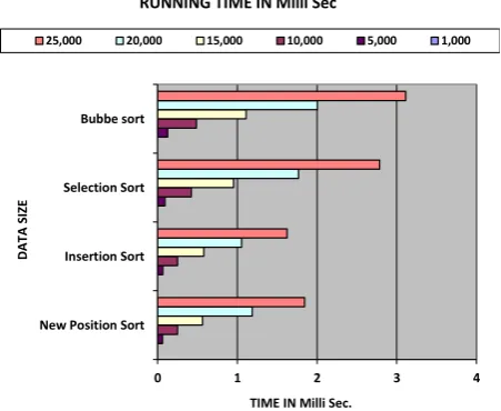
This running time has taken at different-2 data sizes.. We concentrate on the worst-case running time that is longest for any size of input data [1]. Although we can’t find the exact running time because it may be varies. The running time could change according to operating system, processors or compiler also. This running time has been taken by “C free” compiler. And used the header file “#include<time.h>” and use this statement runtime= ((t2-t1) / (double) CLOCKS_PER_SEC); here t1 and t2 is the initial and ending run time respectively. With the help of this we find the running time in milliseconds. We are representing the comparative study of running time between non-recursive comparison based sorting algorithms at worst case.
Fig 2 – Running Time of Various Algorithms
We found the no. of swapping on different data sizes. And found huge differences. As the consult of the worst case, the Position Sort takes the lesser swapping in comparison to other sorting algorithms to perform the sorting operation. Position sort takes the n\2 swapping in the worst case. We show the comparisons of swapping of Position sort, selection sort and bubble sort. We don’t consider the insertion sort here because insertion sort does not swap the elements during the process. Position sort and other these algorithms have a huge difference that’s why Position sort take benefit and perform the process faster.
Fig 3 – No. of Swapping of Various Algorithms
6.
CONCLUSION
We are presenting a unique concept of sorting named as “Position Sort” this method is easy to use, reduce the swapping operation and improve the running time. The concept of Position sort is the easiest and basic concept for performing the sorting. Position sort use the maximum (n-1) swapping to solve the problem. It places the element at its correct position by a single swapping only. We have tried to show the role of swapping in efficiency of sorting algorithms. Basically we consider only no. of comparisons as a key. But we should never forget about swapping also. It helps to increase the efficiency of algorithm by decreasing the no. of swapping. In Future we intended to enhance the running time by reducing the comparisons.
7.
REFERENCE
[1]. T. H. Cormen, C. E. Leiserson, R. L. Rivest, and C. Stein."Introduction to Algorithms" MIT Press, Cambridge, MA, 3rd edition,
[2]. Frank MC (2004). Data Abstraction and Problem Solving with C++. US: Pearson Education, Inc .
[3]. Robert S (1998). Algorithms in C. Addison-Wesley Publishing Company, Inc.
[4]. Box R. and Lacey S., “A Fast Easy Sort,” Computer Journal of Byte Magazine 1991.
[5]. Knuth E., The Art of Computer Programming Sorting and Searching, Addison Wesley, 1998.
0 1 2 3 4
New Position Sort Insertion Sort Selection Sort Bubbe sort
TIME IN Milli Sec.
D
AT
A
SI
ZE
RUNNING TIME IN Milli Sec
25,000 20,000 15,000 10,000 5,000 1,000
0 200000000 400000000
Position Sort Selection Sort Bubble Sort
NO. OF SWAPPINGS
COMPARISONS BETWEEN SWAPPINGS
[image:5.595.58.284.543.728.2][6]. Flores, I. "Analysis of Internal Computer Sorting". J.ACM 7, 4 (Oct. 1960),
[7]. Soubhik Chakraborty, Mausumi Bose, and Kumar Sushant, A Research thesis, On Why Parameters of Input Distributions Need be Taken Into Account For a More Precise Evaluation of Complexity for Certain Algorithms.
[8]. Lipschutz, “Data Structure with C”schaum Series, Tata McGraw-Hill Education.
[9]. V.Estivill-Castro and D.Wood."A Survey of Adaptive Sorting Algorithms", Computing Surveys,
[10].Williams, J.W.J. "Algorithm 232: Heap sort". Comm. ACM 7, 6.