http://dx.doi.org/10.4236/am.2015.65075
Two and Three Dimensions of Generalized
Thermoelastic Medium without Energy
Dissipation under the Effect of Rotation
MohamedI A. Othman1,2, Sarhan Y. Atwa3, Ahmed W. Elwan4
1Department of Mathematics, Faculty of Science, ZagazigUniversity, Zagazig, Egypt 2Department of Mathematics, Faculty of Science, Taif University, Taif City, Saudi Arabia
3Department of Engineering Mathematics and Physics, Higher Institute of Engineering, Shorouk Academy,
Shorouk City, Egypt
4Department of Mathematics, Faculty of Science, King Khalid University, Abha, Saudi Arabia
Email: [email protected], [email protected], [email protected]
Received 29 March 2015; accepted 8 May 2015; published 12 May 2015
Copyright © 2015 by authors and Scientific Research Publishing Inc.
This work is licensed under the Creative Commons Attribution International License (CC BY).
http://creativecommons.org/licenses/by/4.0/
Abstract
The purpose of this paper is to study the effect of rotation on the general three-dimensional model of the equations of the generalized thermoelasticity for a homogeneous isotropic elastic half-space solid. The problem is studied in the context of the Green-Naghdi theory of type II (without energy dissipation). The normal mode analysis is used to obtain the expressions for the temperature, thermal stress, strain and displacement. The distributions of variables considered are represented graphically.
Keywords
Generalized Thermoelasticity, Three-Dimensional Modeling, Rotation, Normal Mode Method, Green-Naghdi Theory
1. Introduction
propagation of heat, these theories involve a hyperbolic heat equation and are referred to as generalized ther-moelasticity theories.
The first generalization, for isotropic bodies, is due to Lord and Shulman [2] who obtain a wave-type heat equation by postulating a new law of heat conduction to replace the classical Fourier’s law. Othman [3] con-structs the model of generalized thermoelasticity in an isotropic elastic medium under the dependence of the modulus of elasticity on the reference temperature with one relaxation time.
The second generalization is known as the theory of thermoelasticity with two relaxation times, or the theory of temperature-rate-dependent thermoelasticity, and is proposed by Green and Lindsay [4]. It is based on a form of the entropy inequality proposed by Green and Laws [5]. It does not violate the Fourier’s law of heat conduc-tion when the body under consideraconduc-tion has a center of symmetry, and it is valid for both isotropic and aniso-tropic bodies. Othman [6] studied the relaxation effects on thermal shock problems in elastic half-space of ge-neralized magneto-thermoelastic waves under three theories.
The theory of thermoelasticity without energy dissipation is another generalized theory and is formulated by Green and Naghdi [7]. It includes the “thermal-displacement gradient” among its independent constitutive va-riables, and differs from the previous theories in that it does not accommodate dissipation of thermal energy. Chandrasekharaiah [8] [9] and Tzou [10] [11] proposed dual-phase-lag thermoelasticity in 1998. A survey of five different thermoelastic models in which disturbances are transmitted in a wavelike manner is due to Het-narski and Ignaczak [12].
The problems for rotating media have also been investigated. Chand et al. [13] presented an investigation of the distribution of deformation, stresses, and the magnetic field in a uniformly rotating homogeneous isotropic, thermally, and electrically conducting elastic half space. Schoenberg and Censor [14], Clarke and Burdness [15], and Destrade [16] studied the effect of rotation on elastic waves. Roychoudhuri and Mukhopadhyay [17] studied the effect of rotation and relaxation times on plane waves in the generalized thermo-viscoelasticity. Ting [18]
investigated the interfacial waves in a rotating anisotropic elastic half space. Othman and Song [19] presented the rotation effect in a magnetothermoelastic medium. Ailawalia and Narah [20] depicted the effects of rotation and gravity in the generalized thermoelastic medium. Othman et al. [21] discussed the effect of magnetic field and rotation on generalized thermo-microstretch elastic solid with mode-I crack under the Green-Naghdi theory.
Recently, Othman et al. [22] discussed the effect of magnetic field on a rotating thermoelastic medium with voids under thermal loading due to laser pulse with energy dissipation. Othman and Atwa [23] studied the effect of rotation on a fiber-reinforced thermoelastic under Green-Naghdi theory and the influence of gravity.
In the present work, we studied the effect of rotation on the general three-dimensional model of the equations of the generalized thermoelasticity for a homogeneous isotropic elastic half-space solid in the context of Green- Naghdi theory of type II without any body forces or heat sources. The effect of rotation on different characteris-tics is shown graphically for generalized thermoelasticity.
2. Governing Equations and Formulation of the Problem
We consider a homogeneous thermoelastic half-space, rotating uniformly with an angular velocity Ω= Ωn, where n is a unit vector representing the direction of the axis of rotation. All quantities considered are func-tions of the time variable t and of the coordinates x, y and z. The displacement equation of motion in the ro-tating frame has two additional terms: centripetal acceleration, Ω∧
(
Ω∧u)
due to time varying motion only and 2Ω∧u where u=(
u v w, ,)
is the dynamic displacement vector, and Ω=(
0, ,0Ω)
.The governing equations of the medium in the context of the generalized thermoelasticity of the Green-Naghdi theory of type IIin the absence of body forces and heat sources are:
Equation of motion:
(
)
{
}
(
2) (
) (
)
2 Tρu+ Ω∧ Ω∧u + Ω∧u = λ µ+ ∇ ∇ ⋅u + ∇ − ∇µ u γ (1)
Heat conduction equation:
2 2
2
0
2 2
E T e
K T C T
t t
ρ ∂ γ ∂
∇ = +
2
ij ekk ij eij T ij
σ =λ δ + µ −γ δ (3) In the preceding equations, λ and µ are Lame’s constant, ρ is the density, σij are the components of the stress tensor, t is the time variable, T is the absolute temperature, γ is a material constant given by
(
3 2)
Tγ = λ+ µ α where αT is the coefficient of linear thermal expansion, K is thermal conductivity, CE is the specific heat at constant strain, T0 is the temperature of the medium in its natural state, assumed to be
such that
(
T T T− 0)
0 1.We can rewrite the equation of motion as
(
)
(
)
2 2 2 2 2 2
2
2 2 2 2 2 2
u u w u u u v w T
t x y x z x
t x y z
ρ∂ − Ω + Ω∂ = λ+ µ ∂ +µ∂ +∂ + λ µ+ ∂ + ∂ −γ ∂
∂ ∂ ∂ ∂ ∂ ∂
∂ ∂ ∂ ∂
(4)
(
)
(
)
2 2 2 2 2 2
2 2 2 2 2
v v v v u w T
x y y z y
t y x z
ρ∂ = λ+ µ ∂ +µ∂ +∂ + λ µ+ ∂ + ∂ −γ∂
∂ ∂ ∂ ∂ ∂
∂ ∂ ∂ ∂
(5)
(
)
(
)
2 2 2 2 2 2
2
2 2 2 2 2 2
w w u w w w u v T
t x z y z z
t z x y
ρ∂ − Ω − Ω∂ = λ+ µ ∂ +µ∂ +∂ + λ µ+ ∂ + ∂ −γ ∂
∂ ∂ ∂ ∂ ∂ ∂
∂ ∂ ∂ ∂
(6)
and the conduction equation takes the form
2 2 2 2 2
0
2 2 2 E 2 2
T T T T e
K C T
x y z ρ t γ t
∂ +∂ +∂ = ∂ + ∂
∂ ∂ ∂ ∂ ∂
(7)
and the stress-displacement-temperature relation as:
2
xx e ux T
σ =λ + µ∂ −γ
∂ (8)
2
yy e vy T
σ =λ + µ∂ −γ
∂ (9)
2
zz e wz T
σ =λ + µ∂ −γ
∂ (10)
xy uy vx
σ =µ∂ +∂
∂ ∂
(11)
xz uz wx
σ =µ∂ +∂
∂ ∂
(12)
yz vz wy
σ =µ∂ +∂
∂ ∂
(13) where
u v w
e
x y z
∂ ∂ ∂
= + +
∂ ∂ ∂ (14) For convenience, we will transform the above equations in non-dimensional forms, so the following non-di- mensional variables are used:
(
)
(
) (
)
(
)
(
)
(
)
(
)
1
1 0 0 0
2
2 2 0
1 2 1 , , , , , , , , , , , , , 2 2 , , , , . 2 ij ij E T T E E C T
x y z x y z u v w u v w t t T
C T T T
C C K C T
K C C C
σ ρ ϖ
ϖ ϖ σ
γ γ
λ µ λ µ γ
ϖ ε
ϖ ρ ρ ρ λ µ
′ ′ ′ = ′ ′ ′ = ′= ′= ′ =
+ +
Ω ′
Ω = = = = =
+
(15)
(
)
2 2 2 2 2 2
2
2 2 2 2 2 1
u u w u u u v w T
t x y x z x
t x β y z β
∂ − Ω + Ω∂ =∂ + ∂ +∂ + − ∂ + ∂ −∂
∂ ∂ ∂ ∂ ∂ ∂
∂ ∂ ∂ ∂ (16)
(
)
2 2 2 2 2 2
2 2 2 2 1
v v v v u w T
x y y z y
t y β x z β
∂ =∂ + ∂ +∂ + − ∂ + ∂ −∂
∂ ∂ ∂ ∂ ∂
∂ ∂ ∂ ∂ (17)
(
)
2 2 2 2 2 2
2
2 2 2 2 2 1
w w u w w w u v T
t x z y z z
t z β x y β
∂ − Ω + Ω∂ =∂ + ∂ +∂ + − ∂ + ∂ −∂
∂ ∂ ∂ ∂ ∂ ∂
∂ ∂ ∂ ∂ (18)
2 2
2 2
2 2
T T T e
C T
t ε t
∂ ∂
∇ = +
∂ ∂ (19)
(
)
2 1 2
xx ux e T
σ = β∂ + − β −
∂ (20)
(
)
2 1 2
yy vy e T
σ = β∂ + − β −
∂ (21)
(
)
2 1 2
zz wz e T
σ = β∂ + − β −
∂ (22)
xy uy vx
σ =β∂ +∂
∂ ∂
(23)
xz uz wx
σ =β∂ +∂
∂ ∂
(24)
yz vz wy
σ =β∂ +∂
∂ ∂
(25)
where 2 2 2 2
2 2 2
x y z
∂ ∂ ∂
∇ = + +
∂ ∂ ∂ , 2
µ β
λ µ
=
+ . From Equations (20)-(22) by addition, we get
e T
σ α= − (26)
where,
3
xx yy zz
σ σ σ
σ = + + , 3 4
3 β
α = − .
We consider plane waves propagating in the plane such that at any instant all the particles in a line parallel to the y axis have equal displacements, i.e. all partial derivatives with respect to y vanish.
We may separate out the purely dilatation and purely rotational disturbances associated with the components u, v and w by introducing the two displacement potentials ϕ and ψ , which are functions of x, y, z
and t, in the form u
(
u v w, ,)
= ∇ + ∇ ∧ϕ ψ , i.e.,
u w
x z z x
ϕ ψ ϕ ψ
∂ ∂ ∂ ∂
= + = −
∂ ∂ ∂ ∂ (27)
and ∇2ϕ= ∇ ⋅ =u e; e is the dilatation, 2 w u
x z
ψ ∂ ∂
∇ = −
∂ ∂ . By using Equation (27) in Equations (16)-(19), we obtain
2
2 2
2 2 t T 0
t
ψ ϕ
∇ − ∂ + Ω + Ω∂ − =
∂ ∂
2
2 2
1 2 1 2 1 0
a a a
t t
ϕ ψ
∇ − ∂ + Ω − Ω∂ =
∂ ∂
(29)
2 2
1 2 0
a v
t ∇ − ∂ =
∂
(30)
2 2
2 2
2 2 3 2 0
a T a
t t
ϕ ∇ − ∂ − ∇ ∂ =
∂ ∂
(31)
where, a1=β1 , 2 2
1 T a
C
= , a3=a2εT.
3. The Solution of the Problem
The solution of the considered physical variables can be decomposed in terms of normal modes as in the fol-lowing form
(
, , , , ,)
(
, , ,)
(
, , , , ,)
( )
e t i ay bz( )ij ij
v T e x y z t v e T x ω
ϕ ψ σ = ϕ ψ∗ ∗ ∗ ∗ ∗σ∗ − + (32)
where i= −1, ω is the angular frequency and a, b are the wave numbers in the y and z-directions, respec-tively and ϕ ψ∗, ∗, , ,v T e∗ ∗ ∗ and
ij
σ∗ are the amplitudes of the field quantities. Using Equation (32), then Equations (28)-(31) take the form
2
2 3 0
D A ϕ∗ Aψ∗ T∗
− + − =
(33)
2
4 5 0
D A ψ∗ Aϕ∗
− − =
(34)
2
6 0
D A v∗
− =
(35)
2 2
7 8 1 0
D A T∗ A D A ϕ∗
− − − =
(36)
where d
d D
x
= , 2
1
A b= , 2 2
2 1
A =A +ω − Ω , A3=2ωΩ, A4 =A a1+ 1
(
ω2− Ω2)
,5 1 3
A =a A , 2
6 1 1
A = A a+ ω , 2
7 1 2
A =A a+ ω , 2
8 3
A =aω .
Eliminating T∗ and ψ∗ between Equations (33), (34) and (36) we get
( )
6 4 2 0
D AD BD C ϕ∗ x
− + − =
(37)
In a similar manner, we can show that ψ∗
( )
xand T x∗
( )
satisfy the equations
( )
6 4 2 0
D AD BD C ψ∗ x
− + − =
(38)
( )
6 4 2 0
D AD BD C T x∗
− + − =
(39)
where
2 4 7 8
A A= +A +A +A ,
(
)
(
)
2 4 7 4 7 8 3 5 1 8
B A A= +A +A A +A +A A A A+ ,
2 4 7 3 5 7 1 4 8
C A A A= +A A A +A A A . Equation (37) can be factored as
(
2 2)(
2 2)(
2 2)
( )
1 2 3 0
D −k D −k D −k ϕ∗ x = (40) where 2
j
( )
3 1 e j k x j j x Mϕ∗ −
=
=
∑
(41)similarly
( )
3 11 e
j
k x j j j
x H M
ψ∗ −
=
=
∑
(42)( )
3 21 e
j
k x j j j
T x∗ H M −
=
=
∑
(43)where 5
1 2 4 j j A H k A =
− and
(
)
(
)
2 8 1 2 2 7 j j jA k A
H
k A
− =
− .
from Equations (41), (42) and (27) then we obtain
( )
3(
1)
j 1 e
j
k x
j j j
u x∗ k ibH M −
=
=
∑
− − (44)( )
3(
1)
j 1 e
j
k x
j j j
w x∗ k H ib M −
=
=
∑
− (45)from Equations (44) and (45) in (14) we get
( )
3(
2 2)
j 1 e
j
k x
j j
e x∗ k b M −
=
=
∑
− (46)from Equations (26), (32), (43) and (46), then we obtain
( )
3(
2 2)
2
j 1 e
j
k x
j j j
x k b H M
σ∗ α α −
=
=
∑
− − (47)4. Application
In order to complete the solution we have to know the parameters Mj, so we will consider the following non- dimensional boundary conditions at the surface x=0 of half space:
a) The thermal boundary condition is
(
0, , ,)
n
q +νT r= y z t (48)
where qn denotes the normal components of the heat flux vector, ν is Biot’s number, and r
(
0, , ,y z t)
re- presents the intensity of the applied heat sources. In order to use the thermal boundary condition (48), we use the generalized Fourier’s law of heat conduction in the non-dimensional form, namelyn T
q
n ∂ = −
∂ (49) From Equations (48), (49) and (29), we get
d on 0
d T
T r x
x
ν ∗− ∗ = ∗ = (50)
b) Mechanical boundary condition:
It is assumed that at x=0, the body is at rest; then the following initial conditions hold:
(
0, , ,)
0, 0, , ,(
)
0, 0, , ,(
)
0u y z t = v y z t = w y z t = . (51)
Using the boundary conditions (50) and (51) in Equations (43)-(45) respectively, we get
(
)
3
2
1 j j j
j
k H M r
ν ∗
=
+ =
(
)
3
1
1 j j j 0
j= k ibH M
− − =
∑
, (53)(
)
3 1
1 j j j 0
j= k H ib M
− =
∑
(54)Solving the system of Equations (52)-(54), we get the parameters M jj
(
=1,2,3)
.3
1 2
1 , 2 , 3
M = ∆ M =∆ M =∆
∆ ∆ ∆ (55)
where
(
)
(
)
(
)
(
)(
)
(
)
(
)
(
)
(
)(
)
(
)
(
)
(
)
(
)(
)
2
1 21 2 3 13 12 2 3 12 13
2
2 22 1 3 13 11 1 3 11 13
2
3 23 1 2 12 11 1 2 11 12
1
1
1 ,
k H k k b H H ib k k H H
k H k k b H H ib k k H H
k H k k b H H ib k k H H
ν
ν
ν
∆ = + − − − − +
− + − − − − +
+ + − − − − +
(
2)
(
)
(
)(
)
1 r∗ k k b2 3 H13 H12 ib k2 k3 1 H H12 13
∆ = − − − − +
(
2)
(
)
(
)(
)
2 r∗ k k b1 3 H13 H11 ib k k1 3 1 H H11 13
∆ = − − − − − +
(
2)
(
)
(
)(
)
3 r∗ k k b1 2 H12 H11 ib k k1 2 1 H H11 12
∆ = − − − − +
5. Numerical Results and Discussions
In order to illustrate the theoretical results obtained in the preceding section, we now present some numerical results. In the calculation process, we take the case of copper material. Since ω is complex, we take
0 i
ω ω= + ζ , where i is the imaginary number. The numerical constants of the problem were taken as: 0.0168
T
ε = , β =0.25, α =0.67, ω =0 2.5, ζ =1, a=0 2. , b=1 2. , ν =50, r∗=100, CT =2.
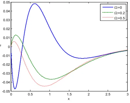
Figures 1-4 represented 2D curves for the change of behavior of the values of the real part of the displace-ment component u, stress σ, strain e and the temperature T against horizontal distance x for y z= =0.9 and t=0.1 for a wide range of x
(
0≤ ≤x 3)
without rotation and with different values of rotation (Ω =0,0.2
Ω = and Ω =0.5). In these figures, the solid line, dashed line and dotted line corresponds for Ω =0, 0.2
[image:7.595.202.427.527.705.2]Ω = and Ω =0.5 respectively, which is furthermore precisely explained in each figure in the legend.
Figure 1displays the distribution of the values of the real part of the displacement component u versus the distance x. The displacement component u always begins from zero for the three values of Ω and satisfies
Figure 1. Displacement distribution at y = z = 0.9.
0 0.5 1 1.5 2 2.5 3
-0.05 -0.04 -0.03 -0.02 -0.01 0 0.01 0.02 0.03 0.04 0.05
x u
Ω=0
Ω=0.2
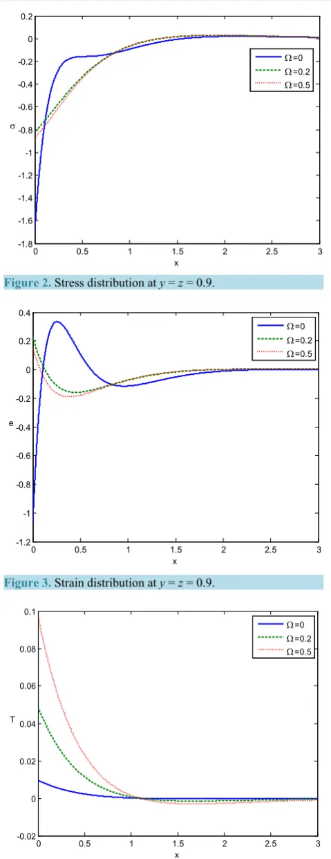
Figure 2. Stress distribution at y = z = 0.9.
Figure 3. Strain distribution at y = z = 0.9.
Figure 4. Temperature distribution at y = z = 0.9.
0 0.5 1 1.5 2 2.5 3
-1.8 -1.6 -1.4 -1.2 -1 -0.8 -0.6 -0.4 -0.2 0 0.2
x
σ
Ω=0
Ω=0.2
Ω=0.5
0 0.5 1 1.5 2 2.5 3
-1.2 -1 -0.8 -0.6 -0.4 -0.2 0 0.2 0.4
x e
Ω=0
Ω=0.2
Ω=0.5
0 0.5 1 1.5 2 2.5 3
-0.02 0 0.02 0.04 0.06 0.08 0.1
x T
the boundary condition at x=0. In the absence of rotation, it is clear that the displacement component u de-creases in the ranges 0≤ ≤x 0.11 and 0.62≤ ≤x 1.87 while it increases in the ranges 0.11≤ ≤x 0.62 and 1.87≤ ≤x 3. In the presence of rotation, the displacement component u increases in the ranges 0≤ ≤x 0.13 and 1.05≤ ≤x 3 for Ω =0.2 and in the ranges 0≤ ≤x 0.08 and 0.88≤ ≤x 3 for Ω =0.5 while it de-creases in the ranges 0.13≤ ≤x 1.05 and 0.08≤ ≤x 0.88 for Ω =0.2 and Ω =0.5 respectively and final-ly all curves converge to zero for sufficientfinal-ly large values of x. It can be observed that the rotational effect de-creases the displacement component u in the range 0≤ ≤x 1.56 and then increases.
Figure 2 represents the variation of stress σ versus the distance x which indicates that all curves start from negative values. It is clear that for absence and presence of rotation all curves increase in the range 0≤ ≤x 2.5 approximately and then starts moving together for x>2.5 and finally converge to the origin. It can be seen that the rotational effect decreases the stress σ .
Figure 3 shows the variation of strain e versus the distance x. It starts from a negative value in the ab-sence of rotation
(
Ω =0)
but it starts form positive values in the presence of rotation(
Ω =0.2, 0.5)
. In the absence of rotation, the strain increases in the ranges 0≤ ≤x 0.26 and 0.84≤ ≤x 2.5 while it decreases in the range 0.26≤ ≤x 0.84. In the presence of rotation, the strain decreases in the ranges 0≤ ≤x 0.46 and 0≤ ≤x 0.39 for Ω =0.2 and Ω =0.5 respectively then increases after that. It is clearly observed that all curves move together in x>2.5 and converge to zero. It can be seen that the rotational effect decreases the strain e in the range 0≤ ≤x 0.84 and then increases.Figure 4 explains the variation of the temperature T versus the distance x. It is clear that all curves begin from positive values. This figure shows that the temperature T decreases in the range 0≤ ≤x 3 and finally all curves converge to zero for sufficiently large values of x It can be observed that the rotational effect increases the tem-perature T in the range 0≤ ≤x 1.1 and then effect decreases.
Figures 5-8are representing 3D surface for curves for distribution of the values of the real part of thedis-placement component u, stress σ , strain e and the temperature T for a wide range of x
(
0≤ ≤x 3)
and for a wide range of dimensionless time t(
0≤ ≤t 0.1)
for y z= =0.9.Figures 9-12 are showing 3D surface for curves for distribution of all physical quantities for a wide range of x
(
0≤ ≤x 3)
and for a wide range of y(
0≤ ≤y 1)
for z=0.9 and t=0.1.All theseFigures 5-12 are in the presence of rotation
(
Ω =0.5)
and they are very important to study the re-lation between physical quantities and dimensionless time t and horizontal distance x and vertical distance y.6. Concluding Remarks
1) The values of the distributions of all physical quantities converge to zero with increasing distance x. Using these results; it is possible to investigate the disturbance caused by more general sources for practical applica-tions.
[image:9.595.183.414.524.699.2]2) It is clearly observed fromFigures 1-4that the rotation Ω plays a significant role in all physical quantities.
Figure 5. Displacement distribution at y = z = 0.9and Ω = 0.5.
0 0.02
0.04 0.06
0.08 0.1
0 1 2 3 -0.05 -0.04 -0.03 -0.02 -0.01 0 0.01
t x
Figure 6. Stress distribution at y = z = 0.9and Ω = 0.5.
Figure 7. Strain distribution at y = z = 0.9and Ω = 0.5.
Figure 8. Temperature distribution at y = z = 0.9and Ω = 0.5.
0 0.02
0.04 0.06
0.08 0.1
0 1 2 3 -1 -0.5 0 0.5
t x
σ
0 0.02
0.04 0.06
0.08 0.1
0 1 2 3 -0.2 -0.1 0 0.1 0.2
t x
e
0 0.02
0.04 0.06
0.08 0.1
0 1 2 3 -0.02 0 0.02 0.04 0.06 0.08 0.1
t x
[image:10.595.192.435.519.699.2]Figure 9. Displacement distribution at z = 0.9, t = 0.1 and Ω = 0.5.
Figure 10. Stress distribution at z = 0.9, t = 0.1 and Ω = 0.5.
Figure 11. Strain distribution at z = 0.9, t = 0.1 and Ω = 0.5.
0 0.2
0.4 0.6
0.8 1
0 1 2 3 -0.06 -0.04 -0.02 0 0.02 0.04
y x
u
0 0.2
0.4 0.6
0.8 1
0 1 2 3 -1.5 -1 -0.5 0 0.5
y x
σ
0 0.2
0.4 0.6
0.8 1
0 1 2 3 -0.2 0 0.2 0.4 0.6
y x
[image:11.595.197.431.514.699.2]Figure 12. Temperature distribution at z = 0.9, t = 0.1 and Ω = 0.5.
3) It is clear fromFigures 5-8 that the changes in the values of the time cause significant changes on all the studied fields.
4) It is observed fromFigures 9-12 that the changes in the values of the dimensions cause significant changes on all the studied fields.
5) The speed of wave propagation of the thermoelastic field variables is finite and coincides with the physical behavior of the elastic materials.
References
[1] Biot, M.A. (1956) Thermoelasticity and Irreversible Thermodynamics. Journal of Applied Physics, 27, 240-253. http://dx.doi.org/10.1063/1.1722402
[2] Lord, H.W. and Shulman Y. (1967) A Generalized Dynamical Theory of Thermoelasticity. Journal of the Mechanics and Physics of Solids, 15, 299-309. http://dx.doi.org/10.1016/0022-5096(67)90024-5
[3] Othman, M.I.A. (2002) Lord-Shulman Theory under the Dependence of the Modulus of Elasticity on the Reference Temperature in Two Dimensional Generalized Thermo-Elasticity. Journal of Thermal Stresses, 25, 1027-1045. http://dx.doi.org/10.1080/01495730290074621
[4] Green, A.E. and Lindsay, K.A. (1972) Thermoelasticity. Journal of Elasticity, 2, 1-7. http://dx.doi.org/10.1007/BF00045689
[5] Green, A.E. and Laws, N. (1972) On the Entropy Production Inequality. Archive for Rational Mechanics and Analysis,
45, 45-47. http://dx.doi.org/10.1007/BF00253395
[6] Othman, M.I.A. (2004) Relaxation Effects on Thermal Shock Problems in an Elastic Half-Space of Generalized Mag-neto-Thermoelastic Waves. Mechanics and Mechanical Engineering, 7, 165-178.
[7] Green, A.E. and Naghdi, P.M. (1993) Thermoelasticity without Energy Dissipation. Journal of Elasticityy, 31, 189-208. http://dx.doi.org/10.1007/BF00044969
[8] Chandrasekharaiah, D.S. (1986) Thermoelasticity with Second Sound: A Review. Applied Mechanics Reviews, 39, 354-376. http://dx.doi.org/10.1115/1.3143705
[9] Chandrasekharaiah, D.S. (1998) Hyperbolic Thermoelasticity: A Review of Recent Literature. Applied Mechanics Re-views, 51, 705-729. http://dx.doi.org/10.1115/1.3098984
[10] Tzou, D.Y. (1995) A Unified Approach for Heat Conduction from Macro- to Micro-Scales. Journal of Heat Transfer,
117, 8-16. http://dx.doi.org/10.1115/1.2822329
[11] Tzou, D.Y. (1996) Macro to Micro-Scale Heat Transfer: The Lagging Behavior. Taylor and Francis, Washington DC. [12] Hetnarski, R.B. and Ignaczak, J. (1998) Approaches to Generalized Thermoelasticity. Taormina Symposium, Italy,
1998, 25-40.
[13] Chand, D., Sharma, J.N. and Sud, S.P. (1990) Transient Generalized Magnetothermo-Elastic Waves in a Rotating Half Space. International Journal of Engineering Science, 28, 547-556. http://dx.doi.org/10.1016/0020-7225(90)90057-P
0 0.2
0.4 0.6
0.8 1
0 1 2 3 -0.05 0 0.05 0.1 0.15
y x
[14] Schoenberg, M. and Censor, D. (1973) Elastic Waves in Rotating Media. Quarterly of Applied Mathematics, 31, 115- 125.
[15] Clarke, N.S. and Burdness, J.S. (1994) Rayleigh Waves on a Rotating Surface. ASME Journal of Applied Mechanics,
61, 724-726. http://dx.doi.org/10.1115/1.2901524
[16] Destrade, M. (2004) Surface Acoustic Waves in Rotating Orthorhombic Crystal. Proceedings of the Royal Society A,
460, 653-665. http://dx.doi.org/10.1098/rspa.2003.1192
[17] Roychoudhuri, S.K. and Mukhopadhyay, S. (2000) Effect of Rotation and Relaxation Times on Plane Waves in Gene-ralized Thermo-Visco-Elasticity. International Journal of Mathematics and Mathematical Sciences, 23, 497-505. http://dx.doi.org/10.1155/S0161171200001356
[18] Ting, T.C.T. (2004) Surface Waves in a Rotating Anisotropic Elastic Half-Space. Wave Motion, 40, 329-346. http://dx.doi.org/10.1016/j.wavemoti.2003.10.005
[19] Othman, M.I.A. and Song, Y. (2008) Effect of Rotation on Plane Waves of Generalized Electro-Magnetothermovis- coelasticity with Two Relaxation Times. Applied Mathematical Modelling, 32, 811-825.
http://dx.doi.org/10.1016/j.apm.2007.02.025
[20] Ailawalia, P. and Narah, N.S. (2009) Effect of Rotation in Generalized Thermoelastic Solid under the Influence of Gravity with an Overlying Infinite Thermoelastic Fluid. Applied Mathematics and Mechanics, 30, 1505-1518. http://dx.doi.org/10.1007/s10483-009-1203-6
[21] Othman, M.I.A., Atwa, S.Y., Jahangir, A. and Khan, A. (2013) Effect of Magnetic Field and Rotation on Generalized Thermo-Microstretch. Elastic Solid with Mode-I Crack under the Green Naghdi Theory. Computational Mathematics and Modeling, 24, 566-591. http://dx.doi.org/10.1007/s10598-013-9200-3
[22] Othman, M.I.A., Zidan, M.E.M. and Hilal, M.I.M. (2014) Effect of Magnetic Field on a Rotating Thermoelastic Me-dium with Voids under Thermal Loading Due to Laser Pulse with Energy Dissipation. Canadian Journal of Physics,
92, 1359-1371. http://dx.doi.org/10.1139/cjp-2013-0689