Software and Hardware Architecture of
H.264/AVC Decoder
Taheni Damak
University of Sousse, Higher Institute of Computerand Communication Techniques, Hammem Sousse,
Tunisia
Hassen Loukil, Ahmed
Ben Atitallah
University of Sfax, Higher Institute of Electronic and telecommunication of Sfax,
Tunisia
Nouri Masmoudi
University of Sfax, National School of Engineering,
Sfax, Tunisia
ABSTRACT
This paper discusses combined software and hardware architecture of a H.264/AVC video compression decoder. The software version of the decoder was implemented using NIOS II processor on a FPGA board (Stratix III of Altera). The mixed, software and hardware, architecture was proposed to ameliorate the decoder speed throughputs. According to the time execution profiling and data dependencies, the decoder partitioning was applied. Thus, the inverse 4x4 Intra process is replaced by a hardware accelerator. It includes inverse 4x4 Intra prediction, inverse transform and inverse quantization. The experimental results at 317 MHz show improvement on the decoding throughput by 20% between software solution and mixed one.
Keywords
H.264 /AVC decoder, software and hardware implementation, inverse 4x4 intra prediction, inverse transform, inverse quantization.
1.
INTRODUCTION
H.264/ AVC [1] codec is a multimedia application that aims at high-quality video contents at low binary rate throughput. H.264 encoder ensures video quality performances by the way of various video coding tools and techniques. In addition, many algorithmic researches are proposed to participate in standard improving in term of quality and bitrates.
While providing a perfect image quality, H.264/AVC requires a reduced execution time. Therefore, architectural researchers and engineering works are made on decoders to respect real time constrains.
The design methodology for realizing a multimedia system on a chip can be roughly partitioned into three axes covering pure software design, pure hardware implementation and mixed software and hardware solution. Software architectures, like work presented in [2], are flexible and take advantage of high design level (data specification level). It is roughly based on processor like RISC CPU or Digital Signal Processor (DSP). However, hardware implementation, e. g. [3] and [4], is more efficient because it can provide parallel tasks execution. But it takes more design time. In addition, it is less flexible then software solution. Examples of hardware boards are FPGA and ASIC. Due to software and hardware solution [5-6-7], both fast development and high performances can be achieved.
In this paper a combined solution is proposed to implement H.264 decoder on FPGA. NIOS II is the used processor. The inverse 4x4 intra chain is the hardware accelerator. The proposed decoder, called LETI decoder, was developed on the basis of H.264 baseline Joint Video Team (JVT) and it was optimized to reduce time execution. Software version of LETI decoder was presented in previous work [2] on DSP platform.
The rest of paper is organized as following: The second section presents related work to introduce the art state of this work. Section 3 details decoder modules to demonstrate complexity of each one. In order to describe proposed implementation solution, section 4 gives the design methodologies in two parts: software implementation and Hardware architecture. Results of hardware implementation are presented in section 5. Then, the results are compared with literature in section 6. The following section (section 7) discuses the validation of the hardware component in SW/HW architecture of H.264 decoder. Finally, a conclusion is presented in section 8.
2.
RELATED WORKS
Research on parallelization of H.264/AVC standard is mostly done for encoders due to their higher performance requirements when comparing to decoders. But data dependencies between blocks and varying macroblock sizes let parallelization more and more difficult. Many works in this axis have been reported in literature. The authors of [8] use pipeline architecture to implement the H.264 encoder with VLSI technology. Other example of hardware encoder implementation is given in [9]. For H.264/AVC decoders, majority of research focuses on CPU specific optimizations and hardware/software combinations. Guan-Yilin et al. [6] present a baseline decoder on ARM966 board, by mixing software optimization and hardware development. The decoder partitioning was done according to the target frame rate and complexity profiles. The hardware acceleration module includes motion compensation, inverse transform and loop filtering. For QCIF video source, the overall throughput is improved by 27%. In fact, a speed improvement leads to 7.4 fps an average.
In [5] also, software / hardware architecture for H.264 baseline profile is proposed, but on single chip decoder SOC. It is called OR264 (OR1K based H264 decoder). The software is used to control the decoding flow. All others blocks are hardware designed and operate in parallel.
In the same research axis, some works use a mixed architecture with an Operating System (OS) as described in [10]. Xenomai is the OS used in [10]. Software part is executed on Power PC hard processor on Xilinx Virtex 5 FPGA. Only deblocking filter is presented as hardware module.
3.
LETI H.264 DECODER STRUCTURE
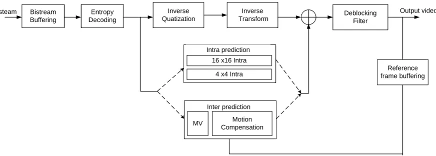
H.264/ AVC [1] video compression standard takes advantage from spatial and temporal redundancy in a video sequence. Therefore, it defines various prediction modes to predict each macroblock depending on its texture properties.In encoder processing, residual macroblocks consists of difference between original macroblocks and the corresponding predicted one. Residual is the final data organized in bitstream. Decoder is responsible to reconstruct a video sequence from the compressed data created by encoder. As shown in Figure 1, first step is entropy decoding. It receives the compressed bitstream to reconstruct video parameters and residual coefficients. Then, two primary paths are considered in decoder process. First one is the decoding of residual macroblocks by inverse quantization and inverse transform. Second path is the generation of the predicted macroblocks according to prediction mode fixed by encoder. The addition of the outputs of these two paths is the reconstruct macroblock. A deblocking filter is then applied to have a better video quality. For more details, following sub-sections describe every module of decoder.
3.1
Entropy decoding
After decoding Network Abstraction Layer (NAL) parameters, the data elements are entropy decoded by two ways: Context-based Adaptive Variable Length Decoding (CAVLD) and Exp-Golomb. CAVLD is used to produce quantized coefficients array. Exp-Golomb is used for others syntaxes elements such as prediction mode and quantization parameter.
CAVLD is more time consuming than Exp-Golomb[11]. It is used to reconstruct and to reorder data on 4x4 block of 16 integers. By the mean of standard code tables, each 4x4 block is decoded into five syntax elements: Coefftoken, Sign, Level, TotalZeros, and Run [1][12].
In last work [13], a software algorithm, called Zero Length Prefix (ZLP), was proposed to optimize Coefftoken step. More than 20% of execution time was reduced. Consequently the decoder time execution was improved. The ZLP algorithm is integrated in this work.
3.2
Inverse quantization
CAVLD output is a residual quantified macroblock. Following step is inverse quantization to produce a set of coefficients (Wij). Since quantization is a losing information
step, inverse quantization reconstructs data. It is a multiplication operation as described in equation 1, where Zij
is inverse quantization input, Wij is its output and Qstep is a
quantization factor given by standard according to Qp value.
Qp is the quantization parameter fixed by encoder. It is decoded from the bitstream using Exp-Golomb codes.
step
ij
ij
Z
Q
W
.
(1)In order to manipulate only integer value in transform step, H.264 standard have postponed real multiplication operation from transform to quantization [12].Details of this operation is given in inverse transform sub section. The final inverse quantization equation given by standard is described by equation 2, where Vij is the rescaling factor defined by the
standard.
To implement this equation, a number of shifts equal to “ floor(Qp / 6)” was used instead of arithmetic multiplication. Shift operation is less time consuming than multiplication operation.
3.3
Inverse transform
In previous video coding standards, Inverse Discrete Cosine Transform (DCT) was used. However, H.264/AVC uses a separable Inverse Integer Cosine Transform (ICT). It has similar properties as a 4x4 inverse DCT [12]. Both DCT and ICT are matrixes multiplication. But they use different matrix coefficients values.
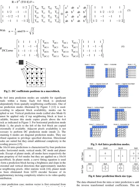
Inverse transform step is applied for each 4x4 block. For 16x16 Intra prediction mode, a suppliant Hadamard transform is adding for DC Coefficients. Most of the energy is concentrated in the DC coefficients for a 16x16 intra coded macroblock. This extra transform helps to de-correlate the DC coefficients to take advantage of the correlation among coefficients. As shown in Figure 2, DC coefficients of each 4x4 block are assembling in a matrix to applied inverse Hadamard transform given by equation 4. An inverse DC quantization is also applied on DC matrix.
3.4
Inverse prediction
Because of redundancy in video sequence, H.264/AVC standard is based on two principal prediction modes [1]. Temporal resemblance between frames is treated as inter prediction. Spatial resemblance in same frame is treated as intra prediction
.
In LETI decoder, first frame of a sequence is necessarily Intra (4x4 or 16x16) coded because it hasn’t reference frame. For next P frames, each macroblock can be coded intra (4x4 or 16x16) or inter prediction.Bistream Buffering
Entropy Decoding
Inverse Quatization
Inverse
Transform DeblockingFilter
Intra prediction
4 x4 Intra 16 x16 Intra
Inter prediction
Motion Compensation MV
Reference frame buffering
[image:2.595.86.522.594.750.2]Output video Bitsteam
Fig 1: H.264/AVC decoder.
)
6
/
(
2
.
.
ij
floor
QP
ij
ij
Z
V
F (T E)F
R T With 5 2 b and 2 1
a
(3)
(4)
0 1 2 3
4 5 6 7
8 9 10 11
12 13 14 15
DC
Fig 2 : DC coefficients positions in a macroblock.
The 4x4 intra prediction modes are suitable for significant details within a frame. Each 4x4 block is predicted independently from spatially neighboring coefficients. One of nine prediction modes illustrated by Figure 3 [12] is used. According to adjacent block availability, modes can be applied or not. Vertical prediction mode (called also Mode 0) cannot be applied only if top neighboring block at least is available, because this mode copies pixels above the 4x4 block as indicated in Figure 3. For horizontal prediction mode (Mode 1), the pixels to the left of the 4x4 block are copied horizontally if available. Adjacent pixels availability is not necessary to perform DC prediction mode (mode 2). The remaining 6 modes are diagonal prediction modes. They use defined equation to privilege specified direction. Directional modes are suited but they entail additional complexity in the decoding process [15].
The 16x16 intra predictions is characterized by four prediction modes: horizontal mode, vertical mode, DC mode and planer mode. Except of planer mode, all modes have respectively the same propriety of 4x4 modes but they are applied on a 16x16 macroblock. In planer mode, a curve fitting equation is used to form a prediction block having a brightness and slope in the horizontal and vertical directions that approximately matches the neighboring pixels. After statistic work [16], planer mode has been eliminated from LETI encoder because of its supplementary incising complexity relative to its video quality contribution.
[image:3.595.60.524.74.699.2]In inter prediction case; motion vector is first extracted from bitstream. Then, motion compensation module is applied. It consists of adding motion vector coordinates to corresponding block in reference frame. Result is reconstructed block. Block size can change from one motion vector to other. Different block sizes are supported in H.264/AVC standard, as shown in Figure 4. In LETI decoder only one frame reference is applied and smaller block size for motion vector is 8x8[17].
Fig 3: 4x4 Intra prediction modes.
0 1 2 3 0
1
0 1
0 1
2 3 0
0 0
1 0 1
16x16 16x8 8x16 8x8
8x8 8x4 4x8 4x4
[image:3.595.327.529.84.663.2]8 x 8 T y p e M B T y p e
Fig 4: Inter prediction block size type.
The data obtained from the intra or inter prediction is added to the inverse transformed residual coefficients. This sum is copied to the decoded buffer which is used as an input for deblocking filter step.
3.5
Deblocking filter
The deblocking filter performs in-loop filtering to reduce blocking artifacts created by image partitioning and quantization. After inverse quantization and inverse
transform, the deblocking filter compares the edge values of each 4x4 block with its adjacent block to select the level of filtering. In LETI decoder, Strong or Standard filter is selected according to the block edge, macroblock position in frame and prediction mode. The design algorithm of deblocking filter used in this work is shown with details in [18].
4.
DESIGN METHODOLOGY
4.1
Software implementation
Inspired by H.264/AVC JM (Joint Model, version 12), the LETI decoder has been developed. It is a baseline decoder with optimized algorithms to overcome standard complexity. Software implementation of LETI decoder was on NIOS II processor, at 160 MHz and with 64 Kbytes cache memory. Synthesis was done on Stratix-III EP3SL150F1152C3 Altera board. Results show that occupied surface is 9 408 ALUTs. It represents 8% of FPGA surface. CIF (352x288) video sequences were successfully reconstructed with a speed of 2.43 fps (frame per second). Qp parameter was fixed to 30. Software implementation was necessary before passing to the mixed implementation to evaluate time execution of each module in decoder. This profiling can give idea about modules complexity. As shown in Figure 5, deblocking filter presents the lion share by 30% of overall decoder time execution. Then inverse quantization and inverse transform have second place by 21%.
The principal aim of our researches is to define software / hardware solution of H.264 decoder. All decoder modules will be designed as hardware IP and only control operations will be done on software part of architecture. To attain this purpose, deblocking filter was first implemented as hardware IP in previous work [18] using ESL tools. The second IP is the subject of this proposed work.
[image:4.595.333.524.116.229.2]In order to have a better partitioning between software and hardware, most demanding modules in term of time execution need to be transformed on hardware accelerator. Despite the importance of time execution, it is not the only constraint to be used to define block that need to be accelerated. Data dependencies and possibility of parallelization in algorithm are also major factors. In fact, inverse quantization, inverse transform and inverse prediction present a good tradeoff between time execution and algorithm constraints. Therefore those three modules have been chosen as hardware IP.
Fig 5: LETI decoder profiling.
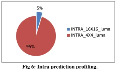
As indicated previously, inverse prediction presents two kinds. In order to define which kind need to be accelerated, a profiling of intra process is made. In Figure 6, time percentage
[image:4.595.54.271.600.713.2]that 4x4 intra and 16x16 intra process take from overall intra time execution in decoder is presented. As clearly shown, 4x4 intra is more used then 16x16 intra.
Fig 6: Intra prediction profiling.
Consequently module accelerator was defined as following: inverse 4x4 intra prediction, inverse quantization and inverse transform for 4x4 intra process.
4.2
Hardware architecture of inverse 4x4
Intra process
Inverse 4x4 intra prediction, inverse quantization and inverse transform are successive decoder modules. Enclosing them in one IP is a way to minimize data transfer between hardware or software part. Architecture of inverse 4x4 Intra chain is given by Figure 7. Accelerator inputs are inverse quantization inputs, prediction modes and macroblock position. Output is only a reconstruct macroblock.
To calculate equations of prediction mode, the inverse 4x4 intra prediction module needs 16 prediction modes and the macroblock position within a frame ( MBX, MBY ). Neighboring pixels are generated by a suppliant component called “Neighboring pixels”.
Inverse quantization process inputs include the CAVLC outputs coefficients of 16 blocks. First of all, coefficients are organized in a 16 coefficients buffer. Then they are sending to inverse quantization component with a control signal. After 16 transfers of 16 coefficients each time, all inputs coefficients of inverse quantization are ready to start execution. For IP output, a buffer is also used to put coefficients by a set of 16. This memory model is used for input and output to minimize memory size. Instead of putting all 256 coefficients in memory waiting bus transfer, only 16 coefficients are waiting. In addition, this option doesn’t affect execution time or transfer time. Details of each module in accelerator are presented in following subsection.
4.2.1 Inverse 4x4 intra prediction
It determinate predicted pixels of all prediction modes in same time. Calculation of each mode is divided on three steps, as illustrated in Figure 8:
-Step 1: The block, called Basic equations, includes commune equations of all prediction modes. Equations are applied using neighboring pixels. Then others equations, called derivate equations, are applied for each corresponding mode. Basic and derivate equations have been generated from standard equations.
- Step 2: The shift module is applied on basic and derivate equation outputs to devise equations respectively by 2 and by 4.
- Step 3: Multiplexer is added to select the corresponding prediction mode, given by Exp-Golomb.
32%
19% 21% 15%
13% deblocking filter
entropy coding
inverse quant_transf
pred_reconst
others
5%
95%
MBX, MBY
Prediction modes
CAVLC outputs coefficients
QP
Input Buffur
Inverse 4x4 quantization
Inverse 4x4
transform
+
Inverse 4x4 Intra prediction Neighboring pixels
Reconstruct Macroblock
[image:5.595.90.510.77.217.2]Output Buffur
Fig 7: Architecture of inverse 4x4 intra process IP.
Basic equations
M U X Reset_0
Clk R_pixels_x x= A:M
8
9
10 11
Capture pixels
Capture res
Basic equations
shifted
Derivate equations
shifted
9 Pred_0_x
x=0:15
Done Control
unit Start
Derivate equations
Shift module
[image:5.595.100.497.97.387.2]Prediction calculation block Pred mode
Fig 8: Inverse 4x4 Intra prediction component.
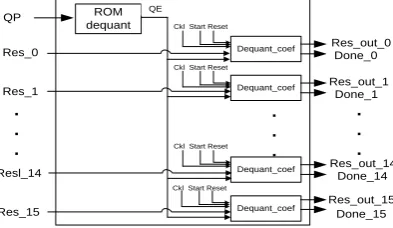
4.2.2 Inverse quantization
Inverse quantization input is 16 coefficients of a block seized 4x4. The proposed implementation takes advantage from hardware parallelism. Inverse quantization of 16 coefficients is trailed in the same time by 16 “Dequant_coef” components as shown in Figure 9. In addition to residual coefficient, clk, reset and start signals, QE parameter is also an input to “Dequant_coef”. QE is a result of Qp parameter divided by 6. As shown in equation 2 in the third section, (Qp/6) appears in inverse quantization equation. Because of division complexity in hardware, a ROM block memory that contains all (Qp/6) possible values has been prepared. In consequence, “ROM dequant” component takes Qp parameter in input and provides QE that presents (Qp/6).
Dequant_coef
ROM
dequant Ckl Start Reset
QE
Res_out_0
Dequant_coef Res_out_1
. . .
. . .
Dequant_coef Res_out_14
Dequant_coef Res_out_15
Done_0
Done_1
Done_14
Done_15 Res_0
Res_1 QP
. . . Resl_14
Res_15
Ckl Start Reset
[image:5.595.323.527.522.650.2]Ckl Start Reset Ckl Start Reset
Fig 9: Inverse quantization component.
Details of “Dequant_coef” components are given in Figure 10. This module is responsible of inverse quantization equation given by equation 2 previously presented. Equation includes multiplication of residual coefficient by Vij parameter.
Vij_ROM in “Dequant_coef” module is a ROM memory block that generates Vij value. MUX block assures Vij and
residual coefficient multiplication. Then a number of QE shifts is applied.
Shift
MUX
Vij_ROM
Control unit Reset
Clk Start
Adress Clk
Clk Start 1
Start 2 Clk Res_in_x
Res_out_x
Done_x
QE
Fig 10: Dequant_coef component.
4.2.3 Inverse transform
[image:5.595.68.265.611.725.2]ICT_1D Clk Reset coef quant_x x=0:15 Start 23 ICT_1D control 9 Coef tran_x x=0:15 Done
Fig 11: Inverse transform component.
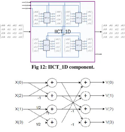
“ICT_1D” component is a 4x4 matrix product. Thus, it consists of four multiplications of the four lines of first matrix by corresponding columns of second matrix. In the proposed design shown in Figure 12, IICT_0, IICT_1, IICT_2, IICT_3 components are implemented to assure the four parallel multiplications.
According to the standard, matrix coefficients are: 1, -1, 1/2 or -1/2. Therefore, no concrete multiplication operation is used. Only right shift, addition and subtraction are applied. Example of column multiplication is presented in Figure 13.
A component for addition is implemented in accelerator to add inverse transform output with predicted coefficients.
[image:6.595.56.276.363.596.2]IICT_0 y0 y3 y1 y2 x0 x3 x1 x2 IICT_1 y0 y3 y1 y2 x0 x3 x1 x2 IICT_2 y0 y3 y1 y2 x0 x3 x1 x2 IICT_3 y0 y3 y1 y2 x0 x3 x1 x2 3 , 3 2 , 3 1 , 3 0 , 3 3 , 2 2 , 2 1 , 2 0 , 2 3 , 1 2 , 1 1 , 1 0 , 1 3 , 0 2 , 0 1 , 0 0 , 0 x x x x x x x x x x x x x x x x 3 , 3 2 , 3 1 , 3 0 , 3 3 , 2 2 , 2 1 , 2 0 , 2 3 , 1 2 , 1 1 , 1 0 , 1 3 , 0 2 , 0 1 , 0 0 , 0 y y y y y y y y y y y y y y y y 3 , 0 2 , 0 1 , 0 0 , 0 x x x x 3 , 1 2 , 1 1 , 1 0 , 1 x x x x 3 , 2 2 , 2 1 , 2 0 , 2 x x x x 3 , 3 2 , 3 1 , 3 0 , 3 x x x x 0 , 3 0 , 2 0 , 1 0 , 0 y y y y 1 , 3 1 , 2 1 , 1 1 , 0 y y y y 2 , 3 2 , 2 2 , 1 2 , 0 y y y y 3 , 3 3 , 2 3 , 1 3 , 0 y y y y IICT_1D reset CLK Done start
Fig 12: IICT_1D component.
Fig 13: IICT_x component.
5.
IMPLEMENTATION AND
PERFORMANCES RESULTS
The designed inverse 4x4 intra block is an IP developed in VHDL language ((VHSIC hardware description language) at the RTL level. It was simulated using Mentor Graphics ModelSim and synthesized using the Altera Quartus II tools. Two different implementations were done for this module by two different technologies: FPGA circuit (Stratix-III EP3SL150F1152C3) [19] and ASIC technology (TSMC 0.18μm standard-cells) [20].
Area cost of inverse 4x4 intra module on Stratix-III seizes only 5 883 ALUTs from a total of 113 600 ALUTs. That
means a percentage of 5% of total FPGA surface. Frequency used is 317.76 MHz. For memory, 1% is only occupied in this work (6 208 bits from 5 630 976 bits). This memory is used for input and output macroblock. For details, synthesis results of each component of the inverse 4x4 intra module and the whole design, on Stratix-III FPGA, are presented in Table.1. It contains the hardware cost in term of ALUTs (Adaptive Look-Up Tables), frequency, block RAM (Random-Access Memory) and block DSP (Digital Signal Processing).
Table 1. Synthesis results on StratixIII.
Modules ALUTs Frequenc y (Mhz) RAM (bits) Block DSP Inverse prediction 580 (<1%)
> 500 0 0 Inverse
quantization
1755 (2%)
340 0 32
(8%) Inverse
transform
1776 (2%)
459 0 0
Addition 288 (<1%)
> 500 0 0 Neighboring 411
(<1%)
440 0 0
Chain Intra 4x4
5 883 (5%)
317.76 6 208 32 (8%)
The lion share component in term of surface is inverse transform and then inverse quantization. Those modules are principal and they can be re-used in inter chain for later implementation. Only inverse quantization uses DSP block because of multiplication operation as given in equation 1 and 2. Prediction module area is the sum of inverse prediction component and neighboring component. Prediction module takes 991 ALUTs. For syntheses on TSMC 0.18 µm technology, results are given in Table 2.
Table 2. Synthesis results of inverse 4x4 intra components on ASIC TSMC 0.18 µm.
Frequency Gates
Inverse Prediction 336.5 Mhz 5706 Inverse quantization 172.5 Mhz 18937
Inverse transform 195.9 Mhz 13199
Addition 531.5 Mhz 2755
Neighboring 387.8 Mhz 3709
Chain Intra 4x4 172.5 Mhz 98505
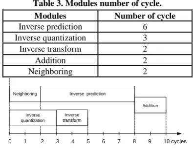
component has 8 cycles of latency. As a result, inverse 4x4 intra module takes 10 cycles to be executed.
Table 3. Modules number of cycle. Modules Number of cycle
Inverse prediction 6
Inverse quantization 3
Inverse transform 2
Addition 2
Neighboring 2
Inverse transform Neighboring Inverse prediction
Addition
0 1 2 3 4 5 6 7 8 9 10 cycles
Inverse quantization
Fig 14 : Running order of inverse 4x4 intra.
6.
COMPARISON WITH PREVIOUS
WORKS
In this section, comparison between the performances of each proposed internal module and the whole inverse 4x4 intra design with other existing designs found in literature (Table 4) are presented. Comparison is not always evident and feasible because of various constrains of designs. Used technology, frequency, voltages and other considerations can change from a work to another.
In term of area consumption, the proposed design improves performances of others works. It takes the lower area in both proposed architectures. In Stratix III case, all blocks are optimized compared to [21], expected of inverse quantization. In 0,18 µm technology, proposed work also offers the better area cost results compared to [5].
The design in [4] is implemented on XilinxC2V1500 board. Only inverse transform and inverse quantization are applied in this work. Those two blocks are compared with the proposed TSMC 0.18μm architecture results because area results are given in kgates. The proposed design is less than 24% of the area occupied by [4]. However, architecture of [4] is faster than the proposed one. The throughput of only inverse transform and inverse quantization of the proposed design is 720 Mpixels/s. It presents less than the half of [4] throughput. To resume, architecture in [4] consume large area to offer better execution speed. In the proposed case, area was reduced to be able to add others H.264 decoder IP in perspective works. In addition, by 360 Mpixels/s, more than 30 frames per second for CIF sequences are decoded. The real time for this module is assured with current throughput. Therefore, proposed throughput results were kept.
Compared to [5], our speed in both technologies is more efficient in term of area and speed.
7.
VALIDATION OF SW/HW
ARCHITECTURE OF H.264 DECODER
After validation of inverse 4x4 intra hardware module separately, it was implemented with software decoder on same board. Proposed co-design architecture is given in Figure 15. The main purpose of software /hardware architecture is to increase the throughput rate of H.264/AVC decoder. The use of a hardware accelerator is an advantage to exploit the parallel and pipelined architectures.Software part is executed on NIOS II soft-core. NIOS II is a 32-bit embedded RISC processor with 6 levels of pipeline. Embedded system communication between processor and accelerator is assured by Avalon bus. It can be seen as a set of predefined signals for connecting one or more IP blocks. The Avalon 32-bits bus provides connection between components masters or slaves. It has a multi-master architecture allowing flexibility in system design.
Avalon bus width is 32- bits. But most accelerator inputs (position parameters, 16 prediction modes and Qp parameters) are defined on only 8 bits each one, as described previously in section 4. To economize time transfer, each 4 parameters have concatenated to send them in one time. Thus, 5 transfers are necessary instead of 19. For residual quantized coefficient, it is defined on 16 bits. They can be sent to accelerator 2 by 2 coefficients. As results, CIF sequence is successfully reconstructed with same PSNR (Peak Signal to Noise Ratio) quality compared with pure software PSNR. Validation was done on bitstreams of several CIF sequences such as Forman and Akiyo. Qp was fixed to 30.
Synthesis results are presented in Table 5. Proposed architecture takes 13.61% of FPGA surface. Occupied memory is 39%. Thus, board capacity allows others accelerator implementations.
Coprocessor Intra 4x4 process
NIOS II CPU
RAM Interface
IRQ controler
A V A L O N
B U S
Timer UART
D
at
a_
in
D
at
a_
ou
t
co
nt
ro
l s
ig
na
ls
Data_out Wait_request
CS Data_in
[image:7.595.323.535.512.622.2]rd/ wr
Fig 15: Embedded system architecture.
Table 4. Results of previous works.
Technology
Occupied area Throughput
Mpixels/s Inverse 4x4 intra
prediction
Inverse quantization
Inverse transform
[4] FPGAXilinxC2V1500 - 135.306 kgates 1586
[5] HW chip 0.18µm 71 kgates 53 kgates 30.3
[21] STRATIX II 37440 LUTs 1151 LUTs 4152 LUTs -
Proposed work
Stratix III 991 LUTs 1776 LUTs 1755 LUTs 360
Table 5. Proposed architecture synthesis results.
Total Pins 201 (27%)
ALUTS number 15.470 (13.61%)
Registers number 12259(9.3 %)
Memory (bits) 2.196.832 (39%)
Blocks DSP number 36 (9%)
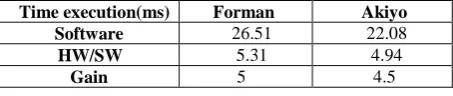
In term of time execution, software intra process takes 26.51ms in one frame of Forman sequence. Concurrently, accelerator is executed in 5.31 ms with transfer time. Despite of transfer time importance, accelerator is faster than software execution by a factor of five. Similar results are proved for Akiyo bitstream. Results are given in details in table 6.
Table 6. Time execution for Forman and Akiyo.
Time execution(ms) Forman Akiyo
Software 26.51 22.08
HW/SW 5.31 4.94
Gain 5 4.5
8.
Conclusion
In this paper, co-design architecture of H.264 decoder was developed. Hardware accelerator is 4x4 intra chain. It contains 4x4 intra prediction, inverse quantization and inverse transform. Hardware design is optimized to assure tradeoff between video time constrain and hardware on chip area. As results, accelerator speed is greater than 20% software speed. In addition, real time for CIF@30frames/s is assured for the proposed accelerator. FPGA area is still available to add other accelerator. Next block to be implemented as hardware IP is Inter prediction. Since inverse transform and inverse quantization which are developed in this work, are the same for intra 4x4 and inter chain, all inter chain will be implemented when design inter prediction block.
9.
References
[1] Wiegand (Ed.), T, “ Draft ITU-T Recommendation H.264/AVC and Draft ISO/IEC 14496-10 AVC”, Joint Video Team of ISO/IEC JTC1/SC29/WG11 &ITU-T SG16/Q.6 Doc. JVT-G050, Mar.
[2] Werda. I, Dammak. T, Grandpierre. T, Ben Ayed MA, Masmoudi N, “ Real-time H.264/AVC baseline decoder implementation on TMS320C6416”, Springer-Verlag 2010, J Real-Time Image Processing.
[3] Warsaw .T, Lukowiak. M, “Architecture design of an H.264/AVC decoder for real-time FPGA implementation”, Application-specific Systems, Architectures and Processors (ASAP'06), 2006 IEEE. [4] Fan C.-P. and Cheng Y.-L., “FPGA implementations of
low latency and high throughput 4x4 block texture coding processor for H.264/AVC”,Journal of the Chinese Institute of Engineers, vol. 32, no. 1, pp. 33–44, 2009. [5] Kun Y, Chun Z, Guoze DU, Jiangxiang XIE, Zhihua W,
“A Hardware-Software Co-design for H.264/AVG Decoder”, Solid-State Circuits Conference, 2006. (ASSCC). IEEE Asian pages : 119-122.
[6] WANG S-H, PENG W-H, “A Software-Hardware Co-Implementation of MPEG-4 Advanced Video Coding
(AVC) Decoder with Block Level Pipelining”, vol. 41, no. 1, pp. 93-110, 2005.
[7] Ben Atitallah A., Kadionik P., Masmoudi N., Lévi H. “Design FPGA implementation of a HW/SW Platform for Multimedia Embedded Systems”, Automation for Embedded Systems Journal, Pages 1-19, Springer 2008. [8] Babionitakis K., Doumenis G., Georgakarakos G.,
Lentaris G., Nakos K., Reisis D., Sifnaios I., Vlassopoulos N., «A real-time H.264/AVC VLSI encoder architecture», Journal of Real-time Image Processing , vol. 3, no. 1-2, pp. 43-59, 2008.
[9] Tran X-T., Tran V-H, “An Efficient Architecture of Forward Transforms and Quantization for H.264/AVC Codecs”, REV Journal on Electronics and Communications, Vol. 1, No. 2, April – June, 2011. [10]Kthiri M., Kadionik P., Le Gal B., Lévi H., Ben Atitallah
A., “Performances analysis and evaluation of Xenomai with a H.264/AVC decoder”, ICM 2011.
[11]Damak T., Werda I., Samet A., Masmoudi N., “DSP CAVLC implementation and Optimization for H.264/AVC baseline encoder”, 15th IEEE International Conference on Electronics, Circuits, and Systems, ICECS 2008, MALTA.
[12]Richardson, I.E.G ,”H.264/AVC and MPEG4 video compression. Video Coding for Next Generatiopn Multimedia”, Wiley editor, 2003.
[13] Damak T., Werda I., Ben Ayad M-A, Masmoudi N, “An Efficient Zero Length Prefix Algorithm for H.264 CAVLC Decoder on TMS320C64”, 2010 International Conference on Design & Technology of Integrated Systems in Nanoscale Era (DTIS).
[14]Malavar, H. Hallapuro, A. Karczewicz, M. Kerofsky, L. “Low complexity transform and quantization in h.264/AVC”, IEEE Transactions on circuit and system for video technology, Vol. 13, No. 7, pp. 598-603, 2003. [15] Soon-kak Kwon, A. Tamhankar, K.R. Rao, “Overview
of H.264/AVC / MPEG-4 Part 10”, Journal of Visual Communication and Image Representation, Vol. 17, No 2 , pp 186–216, Apr. 2006.
[16]Kessentini A., Kaaniche B., Werda I., Samet A., Masmoudi N., “Low complexity intra 16x16 prediction for H.264/AVC” International Conference on Embedded Systems & Critical Applications ICESCA,2008, Tunisia. [17]Werda I., Chaouch H, Samet A, Ben Ayed M-A,
Masmoudi N., “Optimal DSP Based Integer Motion Estimation Implementation for H.264/AVC Baseline Encoder”, The International Arab Journal of Information Technology, Vol. 7, No. 1, January 2010.
[18]Damak T., Werda I., Masmoudi N., Bilavarn S., “Fast prototyping H.264 deblocking filter using ESL Tools”, 2011 8th International Multi-Conference on Systems, Signals & Devices,SSD.
[19]Stratix III device, http://www.altera.com/
[20]Artisan Components. TSMC 0.18μm 1.8-Volt SAGE-XTM Standard Cell Library Databook, 2001.