http://dx.doi.org/10.4236/ojs.2014.49065
How to cite this paper: Janiffer, N.M., Islam, A. and Luke, O. (2014) Estimating Equations for Estimation of Mcdonald Ge-neralized Beta—Binomial Parameters. Open Journal of Statistics, 4, 702-709. http://dx.doi.org/10.4236/ojs.2014.49065
Estimating Equations for Estimation of
Mcdonald Generalized Beta—
Binomial Parameters
Nthiwa M. Janiffer*, Ali Islam, Orawo Luke
Department of Mathematics, Egerton University, Njoro, Kenya
Email: *[email protected], [email protected], [email protected]
Received 4 August 2014; revised 9 September 2014; accepted 25 September 2014 Copyright © 2014 by authors and Scientific Research Publishing Inc.
This work is licensed under the Creative Commons Attribution International License (CC BY).
http://creativecommons.org/licenses/by/4.0/
Abstract
There has been a considerable recent attention in modeling over dispersed binomial data occur-ring in toxicology, biology, clinical medicine, epidemiology and other similar fields using a class of Binomial mixture distribution such as Beta Binomial distribution (BB) and Kumaraswamy-Bi- nomial distribution (KB). A new three-parameter binomial mixture distribution namely, McDo-nald Generalized Beta Binomial (McGBB) distribution has been developed which is superior to KB and BB since studies have shown that it gives a better fit than the KB and BB distribution on both real life data set and on the extended simulation study in handling over dispersed binomial data. The dispersion parameter will be treated as nuisance in the analysis of proportions since our in-terest is in the parameters of McGBB distribution. In this paper, we consider estimation of para-meters of this MCGBB model using Quasi-likelihood (QL) and Quadratic estimating functions (QEEs) with dispersion. By varying the coefficients of the QEE’s we obtain four sets of estimating equations which in turn yield four sets of estimates. We compare small sample relative efficiencies of the estimates based on QEEs and quasi-likelihood with the maximum likelihood estimates. The comparison is performed using real life data sets arising from alcohol consumption practices and simulated data. These comparisons show that estimates based on optimal QEEs and QL are highly efficient and are the best among all estimates investigated.
Keywords
Maximum Likelihood, McDonald Generalized Beta Binomial, Simulation, Quadratic Estimating Equations, Quasi-Likelihood
1. Introduction
Estimating functions have for sometimes been a key concept and subject of inquiry in research and it is known to be the most general method of estimation. The basis of this method is a set of simultaneous equations involv-ing both the data and the unknown model parameters. To obtain an estimator, the estimatinvolv-ing function is equated to zero and then solve the resulting equation with respect to the parameter in order to obtain parameter estimate. Estimating equations are not quite intensive in computation unlike MLEs. Moreover, the MLE estimators are based on the assumption that the distribution is known, however an estimating equation is free of such assump-tions. The usual procedure is to take a parametric model, such as, the McDonald Generalized beta-binomial model to allow over as well as under dispersion and obtain maximum likelihood estimates of the parameters McDonald Generalized Beta Binomial (McGBB) distribution is a three-parameter distribution which is superior to KB in handling over dispersed binomial data. This procedure may produce inefficient or biased estimates when the parametric model does not fit the data well. Alternatively, more robust estimates, such as moment es-timates, quasi-likelihood estimates (Breslow, 1990 [1]; Moore and Tsiatis, 1991 [2]), extended quasi-likelihood estimates (Nelder and Pregibon, 1987 [3]), the Gaussian likelihood estimates (Whittle, 1961 [4]; Crowder, 1985 [5]), estimates based on the pseudo-likelihood estimating equations of Davidian and Carrol (1987) [6] and esti-mates based on quadratic estimating functions of Crowder (1987) [7] and Godambe and Thompson (1989) [8] can be considered. In this paper we consider estimating the parameters of McDonald Generalized Beta Binomial by the quadratic estimating equations (QEE’s) of Crowder (1987) [7] and Godambe and Thompson (1989) [8] and compared the small sample efficiency and bias properties of these estimates with the maximum likelihood estimates. By varying the coefficients of the QEE’s we obtain four sets of estimating equations. We compare the small sample efficiency of the five sets of estimates obtained by the QEE’s and the quasi-likelihood estimates with the maximum likelihood estimates. We compare estimated relative efficiencies of the estimates for two sets of real life data arising from alcohol consumption practices and simulation study. Estimation of the parameters by the six methods is discussed in Section 3. In Section 4 we compare small sample relative efficiencies. This study shows that if interest is on the point parameters then the GL is the method of choice followed by QL.
2. McDonald Generalized Beta-Binomial Distribution of the First Kind
Let p be a random variable following McDonald’s Generalized Beta-Binomial Distribution of the first kind (McDonald, 1984 [9]; McDonald and Xu, 1995 [10]) with three parameters, α, β and γ. The probability density function of p is then given by
(
)
(
)
1(
)
1GB1 ; , , 1 ; 0 1 and , , 0. ,
f p p p p
B
β
αγ γ
α β γ α β γ
α β
γ − −
= − ≤ ≤ > (1)
The th
r moment of the McDonald Generalized Beta-Binomial Distribution of the first kind is given by
( )
(
(
,)
)
. ,
r B r
E P
B r
α β γ α γ
+
= (2)
McDonald Generalized Beta Binomial Distribution
A random variable Y is said to have McDonald Generated Beta Binomial (McGBB) Distribution with para-meter α , β and γ if and only if it satisfies the following stochastic representation. Y p ~ Bin
(
n p,)
and p ~ GB1(
α β γ, ,)
, where α , β and γ are positive real numbers. This distribution was denoted as,Y ~ McGBB
(
n, , , α β γ)
.In general, a Binomial mixture is obtained through an integration approach. Suppose Y follows a binomial distribution given by Bin
(
n p,)
and Y p ~ Bin(
n p,)
. Unconditional PMF of the Y can be obtained by evaluating the integral( )
(
\)
dy Y p p
P y =
∫
P f p Θ p (3)3. Estimation of Parameters of McDonald Generalized Beta-Binomial Distribution
3.1. Maximum Likelihood MethodThe three unknown parameters of McGBB distribution have been estimated using the maximum likelihood es-timation technique. Let Y =
(
y y1, 2,,yN)
be a random sample of size N from a McGBB distribution with unknown parameter vector Θ =(
α β γ, ,)
T, then the log-likelihood function for Θ can be defined as,( )
(
)
( )
0 0 0 0
1
Θ log log log 1 , .
,
k
n y
N N N
j k k
k k k j
n n y y j
l B
y B α β j γ α γ β
− = = = = − = + + − + +
∑
∑
∑
∑
(4)3.2. Quasi-Likelihood
The quasi-likelihood (Wedderburn, 1974 [11]) is based on the knowledge of the form of first two moments of the random variable zi, =Y ni i. Where E z
( )
i, =πi, and var( )
zi, =π(
1−π)
{
1+ −(
n 1)
ρ}
. While with,
i i i
Y =z n then, E Y
( )
=nπi and var( )
Y =nπ(
1−π)
{
1+ −(
n 1)
ρ}
.The quasi-likelihood with the above mean and variance is given by 1
(
, ,)
n
i i i
Q=
∑
=Q z π ρwhere,
(
)
(
)
(
)
{
(
)
}
,
,
, , d .
1 1 1
i i
i i
i i z
i
z t n
Q z t
t t n
π π ρ ρ − = = − + −
∫
By virtue of independence between samples, the quasi-likelihood with the above means and variance is given by:
(
)
(
(
)
{
(
)
)
}
(
)
(
(
)
{
(
)
)
}
,
, ,
, , d and , 1 0,
1 1 1 1 1 1
where 1, , , 1, , , and 0 1.
i i
n
i i i i i i
i i z i j i
j
i i i i i i
z n Q z n
Q z U
n n
i n j k
π π π
π ρ π β ρ
β
π π ρ π π ρ
π = − ∂ − = = = = = ∂ − + − − + − = = ≤ ≤
∑
∫
(5)We denote Equation (5) by λQL. In this case dijβ is given as
(
1)
iij i i ij
j
d β π π π X
β
∂
= = −
∂ . Given
y Z
n
= we
have:
(
)
(
)
(
)
0 1 1 log log 1 1 1 n yQ n y
Z Z n π π ρ = − = + − − + −
∑
where,(
)
(
)
(
(
)
)
(
)
(
)
(
(
)
)
2 2, 2 ,1
, 2 ,1
,1 ,1 ,1 ,1 B B B B B B B B
α β γ α β γ
α γ α γ
α β γ α β γ
α γ α γ
+ + − + + − and 1 , 1 , B B α β γ π α γ + = .
Then the partial derivatives for the three parameters α , β, γ givenρas also obtained as follow:
(
)
(
)
(
(
)
)
(
)
( )
0
1 1 1
1 1 1 n y n y Q y n π
ψ α β ψ α ψ α ψ α β
α = ρ π γ γ
− ∂ = − + + + − + + + ∂
∑
+ − − (6)(
)
(
)
(
(
)
)
(
)
0 1 1 1 1 1 n y n y Q y n πψ α β ψ α β
β = ρ π γ
− ∂ = − + − + + ∂
∑
+ − − (7)(
)
(
)
2 2(
(
)
)
0
1 1 1
. 1 1 1 n y n y Q y n π
ψ α β ψ α
γ = ρ γ γ π γ γ
−
∂ = − + + − +
∂
∑
+ − − (8)
3.3. Quadratic Estimating Equations
(
)
{
(
)
2 2}
i i i i i i i
m
i
gλ =
∑
aλ z −π +bλ z −π +σλ , Crowder (1987) [7], where aiλ and biλ are specified nonsto-chastic functions of λ. Thus, through derivation the unbiased quadratic estimating equations for parameters:
α, β and γ for McGBB distribution is found as follows.
The unbiased quadratic estimating equations for α , β and γ and ρ have the form
(
)
(
)
{
(
)
2 2}
, 0.
j j
n
j i i i i i i i i
U β ρ = aβ z −π +bβ z −π +σλ =
∑
(9)If we take
(
)
(
) (
)
(
) ( )
(
) (
)
2
2 2 2
2 1 2 1
,
2 1 1
1 2
.
2 1 1
j
j
i i
i ij
i i i
i i ij
i
i i i
n a d n d b β λ β λ π β
σ ρ π π
ρ π β
ρ π π σ
− = + − − − − = − −
We obtain the Gaussian estimating equations. We denote this Equation (10) by λ GL
(
)
(
)
(
) (
)
(
)
(
) ( )
(
) (
)
{
(
)
}
2 2 22 2 2 2
1 2 1 2
1
, 0
2 1 1
2 1 1
n i i i i ij
j i ij i i i i i
i i i i i i
n d
n
U d z z λ
λ λ
ρ π β
π
β ρ β π π σ
σ ρ π π ρ π π σ
− − − = + − + − + = − − − −
∑
(10)If we take i j ij2 i d aβ λ β σ
= , and 0
j
i
bβ = .
Then we obtain the unbiased estimating equations (QEE’s) for McDonald Generalized Binomial Distribution. These equations were obtained by combining the quasi-likelihood estimating equations for the regression para-meters and the optimal quadratic estimating equations of Crowder (1987) [7] for the dispersion parameter after setting ϒ1 and ϒ2 to zero.
We denote the estimates so obtained from Equation (11) by λM1
(
)
(
)
{
(
)
2 2}
2
, .
j
n ij
j i i i i i i i
i
d
U z bβ z λ
λ
β
β ρ π π σ
σ
= − + − +
∑
This simplifies to,
(
,)
2(
)
.n ij
j i i i
i
d
U z
λ
β
β ρ π
σ
= −
∑
(11)For
(
)
(
)
( )
(
)
(
)
( )
2 1 2 1 2 2 1 32 1 2 1
1 2 1
, where 2 .
j
j
i i i i i ij
i
i i
i i i i ij
i i i i
i i
d a
d b
λ λ λ
β
λ λ
λ λ
β λ λ λ
λ λ
π σ π π β
σ
π σ π π β
σ
−ϒ + + ϒ − −
=
ϒ
ϒ − − −
= ϒ = ϒ + − ϒ
ϒ
We obtain the optimal quadratic estimating equations. We note that the forms of the skewness ϒ1λ and the kurtosis ϒ2λ are not known. We then take these based on the second, third and fourth moments of the McDo-nald generalized beta-binomial distribution, which are:
(
)
{
(
)
}
(
)
{
(
)
}
(
)
2
3 2
1 1 1 ,
1 2 1 2 1 1 ,
i i i i i
i i i i i
n n
n n
µ π π ρ
µ µ π ρ ρ
= − + −
= − + − +
and
{
(
)
}
{
(
)
}
{
(
)
}
(
){
}
(
)
(
)(
)
4 2 2 2
1 2 1 1 3 1 1 3 1 1
1 3
1 1 1 2
i i i i
i i i i
i i
n n
n n
n
ρ ρ π π ρ
µ µ ρ µ
ρ ρ ρ
+ − + − − − −
= + − +
− + +
We denote the estimates obtained by solving these optimal quadratic estimating equations by λM2 Further we also denote the estimates obtained by solving the optimal quadratic estimating equations with
1iλ 2iλ 0
ϒ = ϒ = by λM3. Note the estimates λM3 are also obtained by using the pseudo-likelihood estimating equations of Davidian and Carrol (1987) [7].
(
)
(
)
(
)
( )
(
)
(
)
(
)
( )
(
)
{
}
1
2 1
2 2
2 3
,
1 2 1 2
2
1 1
0
j
i i i
i ij i ij
n i i i i
i i i i i
i
i i i i
U
d d
z z
λ λ λ
λ λ
λ
λ λ λ λ
β ρ
π σ π σ
β β
π π π π
π π σ
σ σ
ϒ − −
−ϒ + + ϒ −
− −
= − + − + =
ϒ ϒ
∑
(12)[ ]
( ) (
)
(
)
λ(
)
( )
{
(
)
2 2}
2 3
λ λ
1 2 1
2
0 n
i i i ij
ij
i i i i i
i i i i i
d d
z z λ
λ λ
π σ π π β
β
π π σ
σ σ
− − − −
− + − + =
ϒ ϒ
∑
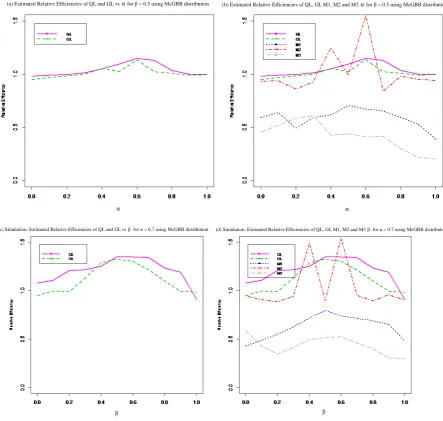
(13)4. Small-Sample Relative Efficiency
The asymptotic relative efficiency may not be very useful when comparing different estimators in small samples. So we conducted a simulation study using relatively small n alongside the real data. We compare the small sample relative efficiency of the estimates obtained by the five estimation procedures: QL; GL; M1; M2;
3
M with the MLE. The estimated Relative efficiency of α is var
(
αML)
var( )
αt where t=QL, GL,1
M , M2, M3. In the situation where relative efficiency is greater than one, then the procedure with its effi-ciency as the denominator is preferred than the “gold standard” ML. The relative efficiency results for the McGBB parameters are summarized inTable 2 for the real data and those for simulated data are summarized in Table 3 andTable 4 and plotted inFigure 1 for simulated data.
[image:5.595.99.541.145.269.2]5. Estimation
Table 1 shows the data set used by Alanko and Lemmens (1996) [12], Rodrίguez-Avi et al. (2007) [13], and Chandrabose et al. (2013) [14] in the study of handling over dispersion. It shows the number of days an individual consumes alcohol y, out of n = 7 days in N = 399, where y = number of days, n = frequency of consumption. We used this data inTable 1 to obtain the estimates for α β, and γ and estimated relative efficiencies by the six different procedures as given inTable 2.
6. Simulation
[image:5.595.87.537.626.715.2]We compare the relative efficiency of the estimates α β, and γ obtained by the six estimation procedures
Table 1.Number of alcohol consumption days and the frequency of consumption.
y 0 1 2 3 4 5 6 7
n 47 54 43 40 40 41 39 95
Table 2.The estimate α β, and γ and their estimated Relative efficiencies by MLE QL M1 M2 and M3 methods for the real data.
Parameter estimates Estimated relative efficiencies
Parameters MLE QL λGL λM1 λM2 λM3 MLE QL λGL λM1 λM2 λM3
α 0.0333 0.0281 0.0301 0.0287 0.0312 0.0282 1.000 1.0912 1.0424 0.6121 0.9352 0.3292
β 0.1797 0.1502 0.1671 0.1655 0.1671 0.1611 1.000 0.9085 0.9831 0.5192 0.9811 0.3615
(a) Estimated Relative Efficiencies of QL and GL vsαfor β = 0.5 using McGBB distribution (b) Estimated Relative Efficiencies of QL, GL M1, M2 and M3αfor β = 0.5 using McGBB distribution
α α
(c) Simulation: Estimated Relative Efficiencies of QL and GL vsβ for α = 0.7 using McGBB distribution
β β
[image:6.595.89.533.86.507.2](d) Simulation: Estimated Relative Efficiencies of QL, GL M1, M2 and M3β for α = 0.7 using McGBB distribution
Figure 1. Plot of relative efficiencies for various estimators relative to that of the MLE under McDonald Generalized Beta- Binomial model: for (a) relative efficiency comparison for α varied when β =0.5 for QL and GL procedures while (b)
α varied when β=0.5 for simulated data for all procedures; for (c) relative efficiency comparison for β varied when 0.7
α = for QL and GL procedures while (d) β varied when α =0.7 for the simulated data for all procedures.
using weekly (7 days) alcohol consumption survey data and simulated data for the survey of weekly alcohol consumption for a small time frame (n=7 days) along with estimates of the parameters of the maximum like-lihood method. Estimated Relative efficiency of α is var
(
αML)
var( )
αt where t=QL, GL, M1, M2,3
M . In the situation where relative efficiency is greater than one, then the procedure with its efficiency as the denominator is preferred than the “gold standard” ML. Using the combination of α β, and γ parameters. We simulated 5000 samples from the MacDonald generalized Beta-Binomial distribution using the weekly al-cohol consumption data. During simulation, all the parameters α β, and γ were estimated for all the six procedures including maximum likelihood and their efficiencies and subsequently their relative efficiencies for the six procedures.Figure 1: Maximum likelihood procedure relative efficiency comparison for (a) when we fix
1
γ = and β=0.5 then α varied for GL and QL procedures, (b) α varied when β =0.5 for all proce-dures. While (c) β varied when α=0.7 and fix γ =1 for GL and QL procedures and (d) β varied when
0.5
7. Discussion
[image:7.595.88.537.272.474.2]FromTable 2, Table 3 andTable 4 we see that the methods QL, GL and M2 all consistently provide high ef-ficiency (never below 0.83). Efef-ficiency of parameters by the method GL is consistently the best. The good be-haviour of the Gaussian likelihood estimator may be due to the fact that the Gaussian likelihood is a proper like-lihood and the distribution of the data does not depend on a specific departure from the binomial distribution. Generally the estimates of parameters by all estimating functions methods have high efficiencies. In this paper we showed that the estimates obtained through small sample parameter estimates and efficiencies obtained dur-ing data analysis are the best for GL followed by QL and then M2 method (estimates based on the optimal quadratic estimating equations with the third and the fourth moments of the McGBB distribution) are consistent. The next best, at the cost of some loss of efficiency, are the M1 and then M3 seems to be the least method. Therefore, when data follow a McGBB distribution, these methods are expected to have high efficiency as compared to MLEs.
Table 3.Relative efficiencies for various estimators for α varied when β=0.5 and γ=1 for simulated data for all procedures.
α varied
Estimated relative efficiencies
MLE QL λGL λM1 λM2 λM3
0.0 1.000 0.980 0.950 0.591 0.933 0.454
0.1 1.000 0.990 0.967 0.638 0.938 0.519
0.2 1.000 0.998 0.985 0.490 0.859 0.586
0.3 1.000 1.014 1.000 0.592 0.928 0.609
0.4 1.000 1.052 1.053 0.617 1.247 0.425
0.5 1.000 1.095 1.025 0.706 0.990 0.438
0.6 1.000 1.148 1.135 0.669 1.552 0.411
0.7 1.000 1.131 1.021 0.655 0.839 0.415
0.8 1.000 1.035 1.010 0.592 0.982 0.298
0.9 1.000 1.001 0.989 0.529 0.952 0.216
1.0 1.000 0.998 0.993 0.389 0.941 0.201
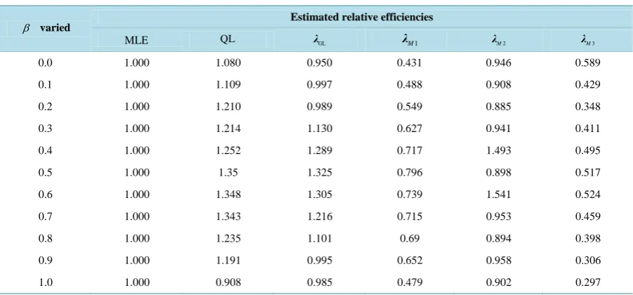
Table 4.Relative efficiencies for various estimators for β varied when α =0.7 and γ=1 for simulated data for all procedures.
β varied Estimated relative efficiencies
MLE QL λGL λM1 λM2 λM3
0.0 1.000 1.080 0.950 0.431 0.946 0.589
0.1 1.000 1.109 0.997 0.488 0.908 0.429
0.2 1.000 1.210 0.989 0.549 0.885 0.348
0.3 1.000 1.214 1.130 0.627 0.941 0.411
0.4 1.000 1.252 1.289 0.717 1.493 0.495
0.5 1.000 1.35 1.325 0.796 0.898 0.517
0.6 1.000 1.348 1.305 0.739 1.541 0.524
0.7 1.000 1.343 1.216 0.715 0.953 0.459
0.8 1.000 1.235 1.101 0.69 0.894 0.398
0.9 1.000 1.191 0.995 0.652 0.958 0.306
[image:7.595.87.538.510.720.2]8. Conclusion
The estimation functions are based on the knowledge of moments and one of the advantages of this approach is that it is robust to model misspecification. The comparison results in this paper indicate that the Estimating Equ-ations are superior to MLE. The small relative efficiency for the estimates results also shows that estimates us-ing optimal quadratic estimatus-ing functions of Crowder (1987) are highly efficient and are the best among all es-timates investigated followed by Quasi-likelihood. Thus, we propose quadratic estimating function for estima-tion of point parameters of any model inclusive of McDonald Generalized Beta-Binomial instead of MLEs since they are consistent and robust to variance misspecification.
References
[1] Breslow, N.E. (1990) Tests of Hypothesis in Over-Dispersed Poisson Regression and Other Quasi-Likelihood Models.
Journal of the American Statistical Association, 85, 565-571.http://dx.doi.org/10.1080/01621459.1990.10476236
[2] Moore, D.F. and Tsiatis, M. (1991) Robust Estimation of the Standard Error in Moment Methods for Extra Binomial/ Extra Poisson Variation. Biometrika, 47, 383-401. http://dx.doi.org/10.2307/2532133
[3] NeIder, J.A. and Pregibon, D. (1987) An Extended Quasi-Likelihood Function. Biometrika, 74, 221-232.
http://dx.doi.org/10.1093/biomet/74.2.221
[4] Whittle, P. (1961) Gaussian Estimation in Stationary Time Series. Bulletin of the International Statistical Institute, 39, 1-26.
[5] Crowder, M.J. (1985) Gaussian Estimation for Correlated Binomial Data. Journal of the Royal Statistical Society,
Se-ries B, 47, 229-237.
[6] Davidian, M. and Carrol, R.J. (1987) Variance Function Estimation. Journal of the American Statistical Association,
82, 1079-1091. http://dx.doi.org/10.1080/01621459.1987.10478543
[7] Crowder, M.J. (1987) On Linear Quadratic Estimating Functions. Biometrika, 74, 591-597.
http://dx.doi.org/10.1093/biomet/74.3.591
[8] Godambe, V.P. and Thompson, M.E. (1989) An Extension of Quasi-Likelihood Estimation. Journal of Statistical
Planning and Inference, 22, 137-152. http://dx.doi.org/10.1016/0378-3758(89)90106-7
[9] McDonald, J.B. (1984) Some Generalized Functions for the Size Distribution of Income. Econometrica: Journal of the
Econometric Society, 52, 647-663. http://dx.doi.org/10.2307/1913469
[10] McDonald, J.B. and Xu, Y.J. (1995) A Generalization of the Beta Distribution with Applications. Journal of
Econome-trics, 66, 133-152. http://dx.doi.org/10.1016/0304-4076(94)01612-4
[11] Wedderburn, R.M. (1974) Quasi-Likelihood Functions, Generalized Linear Models and the Gauss Newton Method.
Biometrics, 61,439-447.
[12] Alanko, T. and Lemmens, P.H. (1996) Response Effects in Consumption Surveys: An Application of the Betabinomial Model to Self-Reported Drinking Frequencies. Journal of Official Statistics, 12, 253-273.
[13] Rodríguez-Avi, J., Conde-Sánchez, A., Sáez-Castillo, A.J. and Olmo-Jiménez, M.J. (2007) A Generalization of the Beta-Binomial Distribution. Journal of the Royal Statistical Society, Series C (Applied Statistics), 56,51-61.
http://dx.doi.org/10.1111/j.1467-9876.2007.00564.x
![Table 1 shows the data set used by Alanko and Lemmens (1996)used this data inChandrabose [12], Rodrίguez-Avi et al](https://thumb-us.123doks.com/thumbv2/123dok_us/8122269.794556/5.595.87.537.626.715/table-shows-data-used-alanko-lemmens-inchandrabose-rodriguez.webp)