Urban Trends and Economic Development in China: Geography Matters!

http://dx.doi.org/10.4236/cus.2014.23016

Urban Trends and Economic Development

in China: Geography Matters!

Michel Dimou, Alexandra Schaffar LEAD-University of Toulon, Toulon, France Email: [email protected], [email protected]

Received 5 June 2014; revised 15 July 2014; accepted 10 August 2014

Copyright © 2014 by authors and Scientific Research Publishing Inc.

This work is licensed under the Creative Commons Attribution International License (CC BY).

http://creativecommons.org/licenses/by/4.0/

Abstract

The aim of this paper is to document the role of spatial effects in the relationship between urban trends and economic development in China, between 1984 and 2004. During this period the Chi-nese urban system experienced dramatic changes, with significant rural-urban, intra-provincial and interprovincial migration, mainly after the 1993 reforms that eased the former Hukou rule and abolished the prevailing cross-region labor mobility restrictions. This study draws upon re-cent econometrical tools based on spatial panel data models, developed in order to deliver evi-dence for a linear relationship between urbanization rates and GDP per capita and an inverted-U relationship between urban primacy and GDP per capita in the Chinese provinces.

Keywords

Urbanization, Urban Primacy, Inverted-U Theories, China

1. Introduction

industrial take-off, economic polarisation and urban concentration; finally during the third stage, high-tech pro-duction leads to diffuse demographical growth.

Using 1950-2050 data, the UN World Urban Prospects (2009) indicate an apparent relationship between the level of economic development and the percentage of urban population. However, this relationship is complex: wealthy regions may have lower urbanization levels, while less developed regions may be associated with higher urbanization rates. Moomaw and Alwosabi (2004) argue that when per capita income level is lower than 1600$, the relationship between the two aggregates is rather loose. It becomes significant above this threshold but be-low 25,000$. Ades and Gleser (1995)introduce institutional factors to explain urbanization patterns, with public transport equipment being among the most important variables. In their comparative study of 85 countries, Da-vis and Henderson (2003) deliver evidence for the role of a country’s political regime on urban primacy.

These studies deliver additional information on the relationship between economic development and urbani-zation but forget its geographical dimension. Wealthy regions or countries with high urbaniurbani-zation rates are often neighbors. Similarly, neighboring poor countries feature same urbanization patterns, with lower urban popula-tion but higher primacy rates. The aim of this paper is to document spatial auto-correlapopula-tion in the relapopula-tionship between urban trends and the GDP/capita level in the Chinese provinces, between 1984 and 2004. During this period, China experienced dramatic changes, with significant rural-urban, intra-provincial and interprovincial migration, mainly after the 1993 reforms that eased the former Hukou rule and abolished the prevailing cross- region labor mobility restrictions. This study draws upon recent econometrical tools on spatial panel data models (Debarsy & Ertur, 2010).

Section 2 focuses on methodological issues. Section 3 delivers the results for the a-spatial models applied on China’s provinces’ economic development and urbanization trends. Section 4 introduces spatial effects. The last section concludes.

2. Methodology

Following Catin et al. (2008), we use 2 equations: the first one determines each province’s urbanization rate (URB), the second one its primacy rate (PRIM), defined as the part of the largest city among all the province’s cities.

Three sets of explanatory variables are used: the first ones determine the level of economic development; the second ones measure the trade openness ratio, reflecting each province’s access to international markets; the third ones concern intra-provinces transport conditions.

Gross Domestic Product (GDPC) per capita features the level of economic development. In order to test the existence of a non-linear relationship between urbanization and the GDP/capita, we also consider a quadratic term for the latter. Changes in GDP/capita may be due to productive accumulation or to global productivity gains without taking into account cross-industry effects in capital accumulation and employment. Non-agricul- tural employment (NAGRI) captures rural-urban migration related to productive accumulation and agriculture- industry transition.

A second set of variables concerns trade openness. The export rate (EXP) captures the ability of the Chinese provinces to interact with international markets. A third set of variables concerns transport equipment within each province. Following Krugman and Livas (1996), we use the railway network density, (TRD) that is the length of the provincial railway network compared to the province’s land area.

Spatial auto-correlation is tested to detect cross-sectional dependence in urbanization and urban primacy re-lated to distance. A battery of tests allows us to discriminate the different spatial models: the spatial autoregres-sive model (SAR) captures possible spatial interaction among the Chinese provinces’ urban trends, the spatial error model (SEM) with a spatial autoregressive parameter of the error term and finally the SARAR model which contains both types of spatial auto-correlation. We present the most robust results, delivered with two different matrices: an inverse distance matrix with dij the distance between the capitals of two provinces i and j;

a contiguity matrix, where two provinces with a common frontier are considered as neighbors.

Data is provided by China’s Annual Statistical Yearbooks. The urban population is considered across the 2000 definition.

3. Results

in 2004. The annual growth rate of GDP per capita was of 8.5% during the 1978-1984 period, 10.2% from 1984 to 1994 and 6.6% from 1994 to 2004. The following Figure 1 delivers information on the correlation between urbanization rate and GDP per capita level. The correlation is much stronger in 2004 than in 1984.

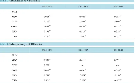
Table 1and Table 2deliver results for both equations (respectively, the dependent variables are the urbaniza-tion rate and the primacy rate) over the whole period, then for each sub-period (1984-1993 and 1994-2004).

Firstly, GDP/capita growth positively impacts urbanization and primacy rates; however there is not a peak- effect, as supposed by Rosen and Resnick. Our findings don’t reveal any inverted-U relationship. The non- agricultural employment is well correlated with urbanization, but much less with urban primacy. Secondly, the railway density is not significant for urbanization. This can be explained by the fact that, once rural workers de-cide to move to the city, transport conditions don’t seem important. TRD is a more accurate variable, when studying urban primacy, since inter-city mobility may affect an urban worker’s locational choices. Thirdly, re-garding model 1, the export rate becomes significant for urbanization after the 1993 reforms and China’s open-ing to foreign investments. All the explanatory variables feature stronger impact on urbanization and urban pri-macy after 1993.

Figure 1. Urbanization rate and GDP/capita in China. Database: CSO (2004).

Table 1.Urbanization vs GDP/capita.

1984-2004 1984-1993 1994-2004

URB

GDP 0.613** _0.408** _0.785**

GDP² 0.033* _0.011* _0.041*

NAGRI 0.643** _0.545** _0.712**

EXP 0.156** _0.118** _0.216**

TRD 0.083* _0.086* _0.077**

Table 2. Urban primacy vs GDP/capita.

1984-2004 1984-1993 1994-2004

PRIM

GDP 0.531** _0.411** _0.671**

GDP² 0.008* _{n.s n.s}

NAGRI 0.411** _0.492** _0.390**

EXP 0.089* _0.078* _0.196*

TRD 0.154* _0.151* _−0.177*

0 1000 2000 3000 4000 5000 6000 7000

0 0.1 0.2 0.3 0.4 0.5 0.6 0.7 0.8 0.9

G

dp

/

c

ap

ita

Urbanization rate

2004

1993

4. Introducing Spatial Dependence

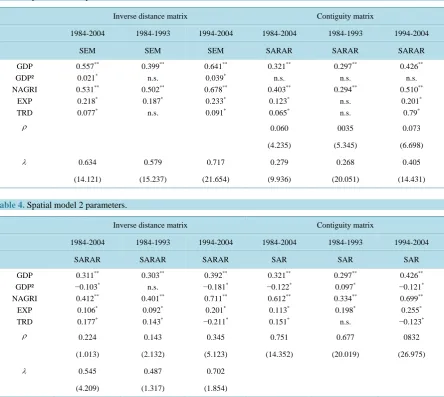
Next, we introduce spatial auto-correlation tests. Conditional hypothesis statistics LM_{λ ρ} and LM_{ρ λ} allow distinction between the alternative specifications for spatial auto-correlation. For the first equation, when the contiguity matrix is used, the null is rejected with both tests for the whole period as well as for each sub-period, which means that the best specification is the SARAR model. When using the inverse distance, the equation for urbanization in the Chinese provinces is best described by a SEM model. For the second equation, when using the inverse distance matrix, the most adequate model is the SARAR; when using the contiguity matrix, the best model is the SAR, which means that when an endogenous spatial lag is included, no residual spatial autocorrela-tion remains.

Table 3 delivers estimations for the spatial autoregressive parameters λ and ρ and for the regression pa-rameters, through the maximum likelihood method.

There is a clear relationship between urbanization and provincial GDP/capita; nevertheless, this relationship doesn’t reveal any inverted-U patterns. Neighboring effects seem stronger after the 1993 reforms. In the SEM model, spatial interdependence relies on spatial diffusion: an exogenous shock (for example the creation of an export process zone) leading to changes in a province’s urbanization affects the neighboring provinces’ urbani-zation rates but the impact of the shock decreases with distance.

Table 4summarizes the results when running the urban primacy regression.

Table 3. Spatial model 1 parameters.

Inverse distance matrix Contiguity matrix

1984-2004 1984-1993 1994-2004 1984-2004 1984-1993 1994-2004

SEM SEM SEM SARAR SARAR SARAR

GDP GDP² NAGRI EXP TRD 0.557** 0.021* 0.531** 0.218* 0.077* 0.399** n.s. 0.502** 0.187* n.s. 0.641** 0.039* 0.678** 0.233* 0.091* 0.321** n.s. 0.403** 0.123* 0.065* 0.297** n.s. 0.294** n.s. n.s. 0.426** n.s. 0.510** 0.201* 0.79*

ρ _{0.060 0035 0.073}

(4.235) (5.345) (6.698)

λ 0.634 0.579 0.717 0.279 0.268 0.405

(14.121) (15.237) (21.654) (9.936) (20.051) (14.431)

Table 4. Spatial model 2 parameters.

Inverse distance matrix Contiguity matrix

1984-2004 1984-1993 1994-2004 1984-2004 1984-1993 1994-2004

SARAR SARAR SARAR SAR SAR SAR

GDP GDP² NAGRI EXP TRD 0.311** −0.103* 0.412** 0.106* 0.177* 0.303** n.s. 0.401** 0.092* 0.143* 0.392** −0.181* 0.711** 0.201* −0.211* 0.321** −0.122* 0.612** 0.113* 0.151* 0.297** 0.097* 0.334** 0.198* n.s. 0.426** −0.121* 0.699** 0.255* −0.123*

ρ _{0.224 0.143 0.345 0.751 0.677 0832}

(1.013) (2.132) (5.123) (14.352) (20.019) (26.975)

λ 0.545 0.487 0.702

There is a convex relationship between the Chinese provinces’ urban primacy rates and the levels of GDP/ capita. The conclusions from the a-spatial model change, mainly after 1993, when the convexity of the relation-ship clearly strengthens: urban primacy follows an ascending trend until a certain level of economic develop-ment, then decreases. TRD is negatively correlated with urban primacy after 1993. Better transport conditions are necessary for demographical dispersion, once a certain threshold of economic development being achieved.

The SAR model implies a global spatial multiplier effect in addition to a spatial diffusion effect of random shocks. Changes in a province’s urban primacy rates multiply the changes occurring in neighboring provinces.

5. Conclusions

The paper examines the determinants of urban trends in China, by introducing spatial dependence effects. Three conclusions may be drawn:

Urbanization is positively correlated with GDP/capita. The introduction of spatial auto-correlation improves the model’s prediction but doesn’t fundamentally modify its conclusions: there are no inverted-U patterns.

Urban primacy is positively correlated with GDP/capita but the conclusions change when we introduce spatial effects: the relationship becomes convex. Urban primacy increases with rural-urban migration when GDP/capita grows until a certain threshold of economic development; once this threshold achieved, urban primacy decreases.

Provincial transport equipment is only relevant for urban primacy, when introducing spatial effects. When ru-ral households move to town, transport issues are not important; however, they become significant when it comes to inter-city migration.

References

Ades, A., & Glaeser, E. (1995). Trade and Circuses, Quarterly Journal of Economics, 110, 195-227. http://dx.doi.org/10.2307/2118515

Catin, M., Hanchane, S., & Kamal, A. (2008). Urbanisation, primate et étapes de développement. Région et Développement, 27, 84-108.

Chinese Statistical Office (CSO) (2004). Chinese Urban Statistical Yearbooks.

Davis, J., & Henderson, V. (2003). Evidence of the Political Economy of the Urbanisation Process. Journal of Urban Eco-nomics,53, 98-123. http://dx.doi.org/10.1016/S0094-1190(02)00504-1

Debarsy, N., & Ertur, C. (2010). Testing for Spatial Autocorrelation in a Fixed Effects panel Data Model. Regional Science and Urban Economics, 40, 453-470. http://dx.doi.org/10.1016/j.regsciurbeco.2010.06.001

Junius, K. (1999) Primacy and Economic Development: Bell Shaped or Parallel Growth of Cities? Journal of Economic De-velopment, 24, 1-22.

Krugman, P., & Livas, R. (1996). Trade Policy and the Third World Metropolis. Journal of Development Economics, 49,

137-150. http://dx.doi.org/10.1016/0304-3878(95)00055-0

MacKellar, F., & Vining, D. (1995). Population Concentration in Less Developed Countries. Papers in Regional Science, 74,

3-30.

Moomaw, R., & Alwosabi, M. (2004). An Empirical Analysis of Competing Explanations of Urban Primacy. Annals of Re-gional Science, 38, 149-171. http://dx.doi.org/10.1007/s00168-003-0137-x

Rosen, K., & Resnick, M. (1980). The Size Distribution of Cities, Journal of Urban Economics,8, 165-186. http://dx.doi.org/10.1016/0094-1190(80)90043-1

United Nations (2009) World Urban Prospects. United Nations, New York.

Wheaton, W., & Shishido, H. (1981). Urban Concentration, Agglomeration Economies and Economic Development. Eco-nomic Development and Cultural Change, 30, 17-30.