An EPQ Model with Power-form Stock Dependent
Demand under Inflationary Environment using
Genetic Algorithm
Chaman Singh
Assistant Professor, Dept. of Mathematics, A.N.D. College (University of Delhi),
Delhi-110019
S. R. Singh
Reader, Dept. of Mathematics, D.N. (P.G.) College, Meerut, U.P. - 250002
ABSTRACT
In this paper a production inventory model for the newly launched product is developed incorporating the effect of inflation and time value of money. The objective of this study is to find the economic production quantities. It is assumed that demand of the items is displayed stock dependent. Production is stopped when the stock-level reached to level Qand Q0 is the
fixed stock-level. In this paper we discussed the following two situations (I) Q Q0 and (II) Q > Q0. Model is formulated to
maximize the total profit. A genetic algorithm with varying population size is used to solve the model. In this GA a subset of better children is included with the parent population for next generation and size of this subset is a percentage of the size of its parent set. Numerical example is given to illustrate the model. Sensitivity analysis with respect to various parameters is also presented.
Keywords:
Genetic Algorithm, Inflation, Stock-dependent demand1. INTRODUCTION
It is well known that the stock level has a motivational effect on the customers in a supermarket; i.e. the demand rate may go up or down if the on-hand inventory level increases or decreases. In corporate world such a situation is known as the stock-dependent demand. It generally arises for a consumer-goods type inventory. In this area a large number of mathematical models have been reported in the existing literature. Among them, to get the idea of the trends of recent research, one may refer to the works of Datta et al.(1998), Balki and Benkherouf (2004), Teng and Chang (2005), Wu et al. (2006), Singh et al. (2007), Singh et al. (2010) and Pareek and Rani (2012) .
Most of the inventory models unrealistically ignore the influence of inflation. This was due to the belief that inflation would not influence the inventory policy to any significant degree. This belief is unrealistic since the resource of an enterprise is highly correlated to the return on investment. The concept of the inflation should be considered especially for long-term investment and forecasting. Among them, to get the idea of the trends of recent research, one may refer to the works of Lieo et al. (2000), Mehta and Shah (2003), Singh and Singh (2010), Singh and Singh (2011).
In the existing literature most of the research papers have been published assuming that the production rate of a manufacturing system is often assumed to be constant while incorporating the stock-dependent demand, but in fact production rate is a variable under managerial control. Production rate may be influenced due to demand, on hand inventory and launching
new competitive product or with the change in customer’s preferences.
In this research paper an EPQ model of an item is developed considering the power form stock-dependent demand under inflation. It is assumed that the production rate is demand dependent. Two situations were discussed in this paper (I) Q Q0 and (II) Q > Q0, where Q is the stock-level at the time production is stopped and Q0 is the fixed stock-level. Model is formulated to maximize the total profit. A genetic algorithm with varying population size is used to solve the model.
2. GENETIC ALGORITHM
Genetic Algorithm is exhaustive search algorithm based on the mechanics of natural selection and genesis (crossover, mutation, etc.). It was developed by Holland, his colleagues and students at the University of Michigan. Because of its generality and other advantages over conventional optimization methods, it has been successfully allied to different decision making problems. To get an idea of recent work on GA, one may refer to the work of Michalewich (1992), Pezzellaa et al. (2008), Golnaz and Reza (2012) and Ramesh and Nanda (2012).
In natural genesis, we know that chromosomes are the main carriers of hereditary factors. At the time of reproduction, crossover and mutation take place among the chromosomes of parents. In this way, hereditary factors of parents are mixed-up and carried over to their offspring. Again, Darwinian principle states that only the fittest animals can survive in nature. So, a pair of parents normally reproduces a better offspring.
taken as fitness of the solution. Evaluate (P(T)) function evaluates fitness of each member of P(T).
2.1. GA Algorithm:
1. Set generation counter T = 0 and maximum generation M = 0
2. Initialize probability of crossover pc, probability of
mutation pm , upper limit of iteration counter M0,
population size N 3. Initialize (P(T )) . 4. Evaluate (P(T)) . 5. While (M < M0 ) .
6. Select N solutions from P(T) for mating pool using Roulette-Wheel process.
7. Select solutions from P(T) , for crossover depending on pc.
8. Make crossover on selected solutions.
9. Select solutions from P(T ) , for mutation depending on pm.
10. Make mutation on selected solutions for mutation to get population P1 (T) .
11. Evaluate (P1 (T )) 12. Set M = M +1
13. If average fitness of P1 (T) > average fitness of P(T) then
14. Set P(T +1) = P1(T ) 15. Set T = T +1 16. Set M = 0 17. End if 18. End While
19. Output: Best solution of P(T) 20. End algorithm.
3. ASSUMPTIONS AND NOTATIONS
Mathematical model in this paper is developed on the basis of the following assumptions and notation.
3.1. Notations:
Following notations have been used in this paperc1 Holding cost of the inventory item, $/
per unit / per unit time c2 Deterioration cost, $ / per unit
c3 Ordering cost, $ / per order
p Production cost, $ / per unit s Selling price, $ / per unit θ Deterioration rate i Inflation rate d Discount rate r = d - i
Q Maximum inventory level of the ordering cycle Q0 Fixed inventory level at which the demand becomes
constant
T
Length of the production cycle I(t) Inventory level at time t [0, T]3.2. Assumptions:
Model is developed under the following assumptions(1) The inventory system involves only one item and the planning horizon is infinite.
(2) Production rate is demand dependent i.e. P(t) = a D(t)
(3) The demand rate D(t) is deterministic and its functional form is given by
I t
, Q Q ,0D t
D , 0 Q Q0
Where > 0, 0 < < 1,
D
Q
0β, and both and are known as scale and shape parameters, respectively.(4) Shortages are not allowed.
4. MODEL FORMULATION
Let the production is stopped when the stock-level reached to level Q, Q0 is the Constant stock-level. Then there may arise the
following two cases
(I) Q Q0 (II) Q > Q0
4.1. Case I: Q Q
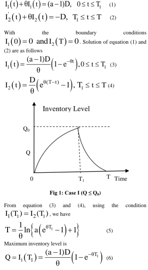
0This is the classical EPQ model for deteriorating items with constant demand rate. Production is started at the time t = 0, with zero inventory level and stopped at the time t = T1 when
the inventory level reaches to the level Q. After that inventory level decreases due to the combined effect of demand and deterioration up to the time T, at which inventory level reaches to the zero level. Inventory level at any time can be described by the following differential equation and graphically represented in the figure-1.
1
1' 1
I t
θ
I t
(a 1)D,
0
t
T
(1)
2
1' 2
I
t
θ
I
t
D,
T
t
T
(2)With the boundary conditions
1
I 0
0
and
I
2
T
0
. Solution of equation (1) and (2) are as follows
1 1
θt
I t
(a 1)D
1 e
,
0
t
T
θ
(3)
2 1
θ(T t)
I
t
D
e
1 , T
t
T
θ
[image:2.595.303.544.323.763.2]
(4)Fig 1: Case I (Q ≤ Q0)
From equation (3) and (4), using the condition
1 1
1 2
I T
( )
I T
( )
, we have
θT1
1
T
ln a e
1
1
θ
(5)Maximum inventory level is
1
1
θT 1
Q
I T
(a 1)D
1 e
θ
(6)T
0 Time
Q
Inventory Level
T1
Present worth holding cost of the inventory held is
1
T rt
1 0 1
HC
c
I (t)e
dt
1
T rt
2
T
I (t)e
dt
(7)Present worth of the production cost is
rT1
paD
PC
1 e
r
(8)Present worth of deterioration cost is
1
T rt
2 0 1
DC
c
θI (t)e dt
1
T rt
2
T
θI (t)e dt
(9)Present worth of sales revenue is
rT
sD
SR
1 e
r
(10)Present worth of ordering cost is
3
OC
c
(11)Present worth of total profit is
1
TP
SR PC HC DC OC
(12)4.1.1. Remark (1):
Using equation (5), we see thatTP
1 is the function of T1 only. Now our problem is to find the optimalvalue of
T
1 in order to maximize the total profit1 1
TP (T )
subject to the inequality constraint Q Q0.Mathematically we have
Maximizing
TP (T )
1 1Subject to Q0Q0, (13)
4.2. Case II:
QQ0In this case production is started at time t = 0, with zero inventory level and stopped at time t = T2 when the inventory
level reached the level Q, where QQ0. Initially the demand and the production rate are constant up to the time t = T1 at
which inventory level reaches to the level Qo after that demand
becomes stock dependent so as the production rate up to the time t = T2. after that inventory level decreases due to the
combined effect of the demand and the deterioration and reaches the zero level at the time t = T. Inventory level at any time can be described by the following differential equation and graphically represented in the figure-2.
1
1' 1
I t
θ
I t
(a 1)D,
0
t
T
(14)
2
2
β' 2
I
t
θ
I
t
(a 1)α
I
t
,
1 2
T
t
T
(15)
3
3
β '
3
I
t
θ
I
t
α
I
t
,
T
2
t
T
3(16)
4
3' 4
[image:3.595.53.237.75.374.2]I
t
θ
I
t
D,
T
t
T
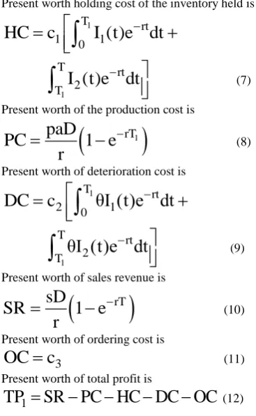
(17)Fig 2: Case II (Q > Q0)
With the boundary conditions
1
I 0
0,
I
2
T
1
Q ,
0I
3
T
3
Q
0and
4
I
T
0
. Solution of equations (14), (15), (16) and (17) are as follows
1 1
θt
I t
(a 1)D
1 e
,
0
t
T
θ
(18)
2
(1 β) 0
I
t
(a 1)α
Q
(a 1)α
θ
θ
1 1 1 θ(1 β)(T t) (1 β)2
T
t
T
e
,
(19)
33
θ(1 β)(T t) (1 β)
0
I
t
Q
α
e
θ
2 1 (1 β) 3T
t
T
α
,
θ
(20)
4 3
θ(T t)
I
t
D
e
1 ,
T
t
T
θ
(21)From equation (18), using the condition
I T
1
1
Q
0, we have1
0
1
(a 1)D
T
ln
θ
(a 1)D Q θ
(22)From equation (19) and (20), using the condition
2 2 3 2
I
T
I
T
, we have
θ(1 β)T23 (1 β)
0
T
1
ln
1
aαe
θ(1 β)
(α θQ
)
(1 β)
θ(1 β)T1
0
θQ
(a 1)α e
(23)From equation (21) using the condition
I
4
T
3
Q
0, we have T 0 QInventory Level
T1 Q0
2
1
θ(1 β)T
4 (1 β)
0
θ(1 β)T (1 β)
0
T
1
ln
1
aαe
θ(1 β)
(α θQ
)
θQ
(a 1)α e
(1 β) 0
1
θ
ln 1
Q
θ
α
(24)Maximum inventory levels is
2 2
(1 β) 0
S
I
T
(a 1)α
Q
θ
1 2
1 (1 β) θ(1 β)(T T )
(a 1)α
e
θ
(25) Present worth of the holding cost is
1 2
1
T rt T rt
1 0 1 T 2
HC c
I (t)e dt
I (t)e dt
3
2 3
T rt T rt
3 4
T
I (t)e dt
TI (t)e dt
(26) Present worth of deterioration cost is
1 2
1
T rt T rt
2 0 1 T 2
DC c
θI (t)e dt
θI (t)e dt
3
2 3
T rt T rt
3 4
T
θI (t)e dt
TθI (t)e dt
(27)Present worth of production cost is
1
T rt
0
PC
p
aDe
dt
2
1
T β rt
2
T
aα I (t)
e dt
(28)Present worth of sales revenue is
1 2
1
T rt T β rt
2
0 T
SR sα
De dt
I (t) e dt
32 3
T β rt T rt
3
T
I (t) e dt
TDe dt
(29)Present worth of ordering cost is
3
OC
c
(30) Present worth of total profit is2
TP
SR PC HC DC OC
(31)4.2.1. Remark (2):
Using equation (22), (23) and (24), we see thatTP
2 is the function of T2 only. Now our problem is tofind the optimal value of T2 in order to maximize the total profit
2 2
TP (T )
subject to the inequality constraintQ
Q
0. Mathematically we haveMaximizing
TP (T )
2 2Subject to
Q Q
0
0, (32)5. NUMERICAL ILLUSTRATIONS
5.1. Case I:
Q
0 Q
:
The following numerical data are used to illustrate the model.
a = 1.2, α = 25, β = 0.25, Q0 = 150, c1 = 0.5, c2 = 0.4, c3 = 200,
p = 5, s = 9, d = 0.1, i = 0.05, r = 0.05, θ = 0.01
For the above assumed parametric values the results are obtained using GA and results are presented in Table 1. It is found that optimal cycle length T = 10.66, maximum inventory level Q = 149.99 units, production time T1 = 8.96 and the
present value of the optimal profit is 2219.12. So at the beginning of each cycle the manufacturer produce the items at a rate P for the period T1 = 8.96. During this period inventory is
built up at the rate P – D – θ I(t), and at time t = 8.96 inventory level reaches149.99 units. At this time the manufacturer stops production and inventory depleted due to the combined effect of demand and deterioration. Inventory level reaches zero level at time t = 10.66, then production for next cycle starts.
5.2. Sensitivity analysis, Case I:
Q
0Q
: variation of the total profit w.r.t. different parameters and results are presented in the table 2, 3, 4 and 5.5.3. Case II:
QQ0Using the same data as in case-I, results are obtained using GA and presented in Table 6.
It is found that optimal cycle length T = 38.21, maximum inventory level Q = 574.38 units, production time T2 = 32.67
and the present value of the optimal profit is 12813.90. So at the beginning of each cycle the manufacturer produce the items at a rate P for the period T1 = 32.67. During this period inventory is
built up and at time t = 32.67, inventory level reaches 574.38 units. At this time the manufacturer stops production and inventory depleted due to the combined effect of demand and deterioration. Inventory level reaches zero level at time t = 38.21, then production for next cycle starts.
5.4. Sensitivity analysis for Case II: QQ0: variation
of the total profit w.r.t. different parameters and results are presented in table 7, 8, 9 and 10.
5.5. Observations:
For the above parametric values optimal profit due to different production rates are obtained and presented in table 2 for case I and in table 7 for case II. From Table 1, it is observed that optimal profits decrease as production rate increases. It happens because increase in production rate, increased stock level and hence increases the holding cost. The increased holding cost dominates the profit due to increases demand hence profit decreases. From Table 7, it is observed that optimal profits increase as production rate increases. It happens because increase in production rate increases stock level and as demand is stock dependent, increased stock level increases the demand of the item, which in turn increases the profit. But increase in stock level increases the holding cost. Profit due to increased demand dominates the loss due to increased holding cost. Thus increase in the production rate increases optimal profit.
Results are obtained for the above parametric values and different values of ‘resultant effect of inflation and discount rate’ r, and presented in the table 5 for case I and in table 10 for case II. It is observed that profit decreases with increase of r, which agrees with reality.
5 10 15 20 25 30
[image:5.595.320.529.70.234.2]500 1000 1500 2000 2500 3000
Fig 3: Total profit with respect to T1 for Case I
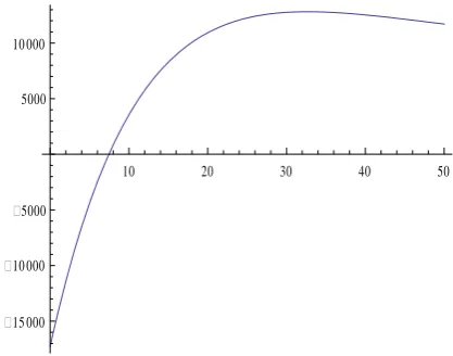
10 20 30 40 50
15 000 10 000 5000 5000 10 000
Fig 4: Total profit with respect to T2 for Case II
6.
CONCLUSIONS AND FUTURE
RESEARCH
In this paper, an EPQ model has been considered under inflation and time discounting over an infinite horizon. Some interesting observations are presented. Demand is taken as the power form stock dependent and the production is taken as the demand dependent. In this paper we discussed the following two cases (I) Q Q0 and (II) Q > Q0, where Q is the stock-level
at the time production is stopped and Q0 is the fixed stock-level.
Model is formulated to maximize the total profit. Also a genetic algorithm with varying population size is used to solve a production inventory model. It is found that this GA is efficient in solving the proposed inventory model. This GA can also be used to solve different decision making problems in different fields of science and technology. This inventory model can be extend incorporating price dependent demand, trade credit policy, two warehouse, etc.
Table 1: Optimal results for Case I:
Q
0 Q
T1 T Q TP1(T1)
8.96 10.66 149.99 2219.12
Table 2: Present value of total profits of the model due to different production rates for Case I
a 1.1 1.3 1.4 1.5 1.6 1.7 1.8
TP1 3605.77 1639.64 1324.81 1127.46 992.27 893.89 819.11
Table 3: Present value of total profits of the model due to different demand parameter “α” for Case I
α 21 22 23 24 26 27 28
TP1 2042.29 2091.09 2136.67 2179.26 2256.51 2291.65 2324.72
Table 4:Present value of total profits of the model due to different demand parameter “β” for Case I
β 0.21 0.22 0.23 0.24 0.26 0.27 0.28
TP1 2014.26 2067.61 2119.55 2170.06 2266.73 2312.88 2357.57
Table 5:Present value of total profits of the model due to different „r‟ for Case I
r 0.046 0.047 0.048 0.049 0.051 0.052 0.053
TP1 2276.22 2261.77 2247.44 2233.23 2205.13 2191.24 2177.47
Table 6:Optimal results for Case II: QQ0
T1 T2 T3 T4 Q TP2(T2)
[image:5.595.53.283.144.310.2]Table 7:Present value of total profits of the model due to different production ratesfor Case II
a 1.1 1.3 1.4 1.5 1.6 1.7
TP1 7127.14 19566.90 26545.10 33545.80 40504.10 47398.70
Table 8:Present value of total profits of the model due to different demand parameter “α” for Case II
α 21 22 23 24 26 27
TP1 9287.83 10134.10 11004.60 11898.10 13751.00 14708.60
Table 9:Present value of total profits of the model due to different demand parameter “β” for Case II
β 0.21 0.22 0.23 0.24 0.26 0.27
TP1 6694.48 7826.87 9188.04 10829.10 15222.20 18154.60
Table 10:Present value of total profits of the model due to different „r‟ for Case II
r 0.046 0.047 0.048 0.049 0.051 0.052
TP1 14082.10 13747.30 13424.80 13113.80 12524.40 12244.80
7. REFERENCE
[1] Balkhi, T.Z., Benkherouf, L. 2004. On an inventory model for deteriorating items with stock dependent and time varying demand rates. Computers and Operations Research 31, 223-240.
[2] Datta T.K., Paul K., Pal A.K. 1998. Demand promotion by up-gradation under stock-dependent demand situation – a model. International Journal of Production Economics, 55, 31–38.
[3] Golnaz H. and Reza M. B. 2012. Using genetic algorithm for fuel consumption optimization of a natural gas transmission compressor station. International Journal of Computer Applications 43(1):1-6.
[4] Liao H.C., Tsai C-H, Su C.T. 2000. An inventory model with deteriorating items under inflation when a delay in payment is permissible, International Journal of Production Economics, 63, 207-214
[5] Mehta N.J. and Shah N.H. 2003. An inventory model for deteriorating items with exponentially increasing demand and shortages under inflation and time discounting, Investigacao Operacional, 23, 103-111.
[6] Michalewicz, Z. 1992, Genetic algorithms + data structures = evolution programs. Berlin: Springer.
[7] Pareek, Sarla and Rani, Sujata. 2012. Supply chain inventory model for deteriorating items with stock dependent demand under progressive trade credit scheme. ASOR Bulletin 31(1), 23 – 35.
[8] Pezzella, F., Morgantia, G., Ciaschettib, G. 2008, A genetic algorithm for the flexibile job-shop scheduling problem, Computers and Operations Research 35, 3202-3212.
[9] Ramesh T k Babu and Nanda Dulal Jana. 2012. An optimized way for static channel allocation in mobile networks using Genetic algorithms. International Journal of Computer Applications 45(19):48-52.
[10] Singh, S. R., Singh, C., Singh, T.J. 2007. Optimal policy for decaying items with stock-dependent demand under inflation in a supply chain, International Review of Pure and Applied Mathematics, 3(2), 189-197.
[11] Singh, S. R., Kumari, R., Kumar, N. 2010. Replenishment policy for non-instantaneous deteriorating items with stock-dependent demand and partial back logging with two-storage facility under inflation. International Journal of Operations Research and Optimization, 1(1), 161-179.
[12] Singh, S. R., Singh, C. 2010. Two echelon supply chain model with imperfect production, for Weibull distribution deteriorating items under imprecise and inflationary environment. International Journal of Operations Research and Optimization, 1(1), 9-25.
[13] Singh, C. and Singh, S. R. 2011. Imperfect production process with exponential Demand rate, Weibull deterioration under inflation. International Journal of Operational Research, 12(4), 430-445.
[14] Teng, J.T. and Chang, C.T. 2005. Economic production quantity models for deteriorating items with price and stock dependent demand. Computers and Operational Research 32, 297-308.