Relative Superior Julia Sets for Complex
Carotid-Kundalini Function
Priti Dimri
Associate Professor,
Department of Computer
Science and Engineering,
G.B Pant Engineering College,
Pauri Garhwal, 246001
Ashish Negi
Associate Professor,
Department of Computer
Science and Engineering,
G.B Pant Engineering College,
Pauri Garhwal, 246001
Udai Bhan Trivedi
Associate Professor
Department of Computer
Science, IMS, Dehradun
ABSTRACT
Carotid Kundalini function broadly known as C-K function was introduced by Gordon R.J.Cooper. It is given by the
function
1
1
cos(
cos ( ))
n n n
z
Nz
z
c
where z,c andN are complex constants. Cooper presented interesting Julia sets by taking c=(0,0).Rani and Negi introduced a new process for generation of the C-K function and obtained interesting variants of Julia set generated by Cooper an some exciting
figures for parameter
N
2
, for values of c other than (0, 0). In this paper we apply a different iteration process for generation of the Julia set for C-K function and will call them relative superiorC-K Julia sets. Further, different properties like trajectories and fixed point arealso discussed in the paper. We also obtain some exciting figures for the C-K function for values of c other than (0, 0).General Terms
Your general terms must be any term which can be used for general classification of the submitted material such as Pattern Recognition, Security, Algorithms et. al.
Keywords
Carotid Kundalini function, Ishikawa iteration, Relative superior C-K Julia set.
1.
INTRODUCTION
In mathematics the Mandelbrot set, named after Benoit Mandelbrot, is a set of points in the complex plane, the boundary of which forms a fractal. Mathematically, the Mandelbrot set can be defined as the set of complex values of c for which the orbit of 0 under iteration of the complex
quadratic polynomial
2 1
n n
z
z
c
remains boundedsee[1-16]. Julia sets [13] provide a most striking illustration of how an apparently simple process can lead to highly intricate sets. Function on the complex plain
c
as simple as2 1
n n
z
z
c
give rise of fractals of exotic appearance. Using other functions in place of this function yield Julia sets of different kinds.
One such function is Carotid-Kundalini function given
by
1
1
cos(
cos ( ))
n n n
z
Nz
z
c
where N and c are
parameters and
cos( )
2
iz ize
e
z
. This function falls under the category of transcendental functions, the study ofwhich was initiated by Fatou[10]. Points with unbounded orbits are not in Fatou sets but they must lie in Julia sets. Attractive points of a function have a basin of attraction, which may be disconnected. A point z in Julia for cosine
function has an orbit that satisfies
Im( )
z
50
.The iteration of complex analytic function F decomposes the complex plane into two complementary sets:
Julia set, which consists of values with the property such that an arbitrarily small perturbation can cause drastic changes in the sequence of iterated function values. The iteration on the Julia set exhibits „chaotic‟ behaviour, &
Fatou set, which consists of values with the property that all nearby values behave similarly under repeated iteration of the function. The iteration on Fatou set exhibits a “regular” behaviour.
Günter Rottenfußer, Dierk Schleicher[14] showed that the escaping points which converge to
under iteration of cosine functions are organized in the form of dynamic rays and, as in the exponential family, every escaping point is either on one of these rays or the landing point of a unique ray. It is well known that the set of escaping points is an open neighbourhood of
, which can be parameterized by dynamic rays. For the entire transcendental functions, the point
is an essential singularity (rather than super attracting point). Eremenko[9] studied that for entire transcendental functions, the set of escaping points is always non-empty. R.L. Devaney, see [3-7], provided answers to his queries, for the special case of exponential function, where every escaping point can be connected to
, along with unique curve running entirely through the escaping points.A dynamic ray is connected component of the escaping set, removing the landing points. It turns out to be union of all uncountable many dynamic rays, having Hausdorff dimension equal to one. However, by a result of McMullen[15], the set of escaping points of a cosine family has an infinite planar Lesbegue measure. Therefore, the entire measure of escaping points sits in the landing points of those rays which land at the escaping points.
Recently, many cosine functions of the following forms have been considered by various researchers, see[20,22-25]:
cos(
z
n
c where
),
n
2
( )
(
iz iz) / 2
In this paper we have usedthe cosine function of the type 1
1
cos(
cos ( ))
n n n
z
Nz
z
c
where N and c areparameters and
cos( )
2
iz ize
e
z
. This function is also known as Carotid- Kundalini(C-K) function [1, 2, 24 ]. When the C-K equation which is given by:1 ,
( )
n n c n
z
K
z
(1)Where n= number of iterations, is iterated, many fascinating properties are revealed as given by Cooper[1-2].By using the above equation, Cooper produced a range of fractal Julia sets in the complex plane as parameters c and N were varied [2]. Also periodic behaviour was observed in some trajectories that remained bounded. Recently, Rani and Negi [17] studied the C-K equation by using superior iterates given by:
1
(
,(
))
(1
)
n n c n n
z
s K
z
s z
(2)
where
0
s
1
.Following Rani and Kumar [11], the orbit generated by equation (2) was called the superior iterations. In this paper we have applied a new iteration process i.e. Ishikawa iteration to the C-K function given by:
,
1 ,
( ( )) (1 ) ( ( )) (1 )
n n n c n n n
n n n c n n n
y s K z s x
x s K y s x
(3)
where
0
s
n
1, 0
s
n1
ands s
n,
n
are convergent to non zero number.Following the study of Rana et. al. [19], the orbit generated by the equation (3) will be called relative superior orbit. Julia sets may be computed for any complex map. In this paper, we focus our study on Julia sets for Carotid-Kundalini(C-K) functions using Ishikawa iterates. We obtain new C-K Julia sets using relative superior Iterates. Here we have used different valuesof the new parameter s‟ and the values for the parameter N, c and s will be taken as taken by Rani and Negi.[17]
2.
PRELIMINARIES
The process of generating a fractal image
from
1 1 cos( cos ( ))
n n n
z Nz z c consists of
iterating the function up to n time‟s see [23].
Definition2.1: Ishikawa Iteration [16]: Let X be a subset of
real or complex numbers and f :X X .For x0X,
we have the sequences
x
nand y
n in X in the following manner:1
(
)
(1
)
(
)
(1
)
n n n n n
n n n n n
y
s f x
s
x
x
s f y
s
x
where
0
s
n
1,
0
s
n
1,
{ }
s
n
&{ }
s
n are convergentto non zero number
Definition 2.2[18, 19]: The sequence of {xn} and
{
y
n}
described above is called the Ishikawa sequence of
iterations or Relative Superior sequences of iterates. We
denote it by
RSO x s s t
( , , , )
o n n
. Notice that( , , , )
o n nRSO x s s t
with
s
n
1
is SO x( o,sn, )t i.e.Mann orbit and if we place
s
n
s
n
1
then( o, n, ' , )n
RSO x s s t reduces toO x t( o, ). The set of points whose orbits are bounded under relative superior
iteration of the function
f z
( )
is called Relative Superior Julia sets.Definition 2.3[18, 19] Relative superior C-K sets for the
function
1 1
cos(
cos (
))
n n n
z
Nz
z
c
where
n=1,2,3,… is defined as the collection of
c C
for which the orbit of 0 is bounded.The collection of points that are bounded, i.e. there exists M,
such that| ( ) | n
Q z M , for all n, is called as a prisoner set
while the collection of points that are in the stable set of infinity is called the escape set. Hence, the boundary of the prisoner set is simultaneously the boundary of escape set and that is Julia set for Q.
Definition 2.4 [18, 19]: The set of points whose orbits are bounded under relative superior iteration of the function Q (z) is called Relative Superior Julia sets.
3.
GEOMETRY
OF
RELATIVE
SUPERIOR JULIA SETS FOR C-K
FUNCTION
The fractals generated from the
equation
1 1
cos(
cos (
))
n n n
z
Nz
z
c
showssymmetry along the real axis for both Real and Imaginary values:
a) When the powers of eq2 and function3 is kept constant and the power of first function is varied then the following properties of composite fractal us as found as follows:
a. At p=2,q=2,r=2 , we observe that the composite fractal exhibits symmetry across the real axes i.e. x-axis and there are 5 petals each of which contains 4 mandelbrot sets of order 2 . The fifth petal contains the fractal similar to mandelbar. This fractal contains a tail.
b. All the petals contains one of infinite Mandelbrot sets contained within all the petals of the composite fractal.
b) For all the imaginary values we observe that the relative superior C-K Julia set consists of disjoint curves (hairs) tending to infinity in all the three arms.
4.
GENERATION
OF
RELATIVE
SUPERIOR
CAROTID-KUNDALINI
[image:2.595.53.284.73.191.2]SETS
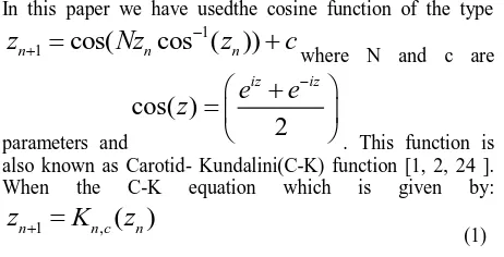
Fig4.2: Relative Superior C-K set for N=(1,0), s=0.5 and s’=0.5
Fig. 4.3: Relative Superior C-K set for N=(1,0), s=0.1 and s’=0.1
Fig 4.4: Relative Superior C-K set for N=(0,0.7), s=0.0 and s’=0.1
Fig. 4.5: Relative Superior CK set for N=(3,0), s=0.5 and s’=0.5
[image:3.595.75.271.75.216.2]Fig. 4.6: Relative Superior CK set for N=(5,0), s=0.1and s’=0.1
Fig. 4.7: Relative Superior CK set for N=(0,3), s=0.1 and s’=0.04
Fig.4.8: Relative Superior CK set for N=(0,14.5), s=0.01 and s’=0.01
5.
GENERATION
OF
RELATIVE
SUPERIOR
CAROTID-KUNDALINI
JULIA SETS
Fig 5.1: Relative Superior C-K Julia set for c=(0,0) at N=(0.02,0), s=0.5 and s’=0.5
Fig 5.2: Relative Superior C-K Julia set for c = (-0.03588, 0.01962) at N=(1,0) ,s=0.5,s’=0.5
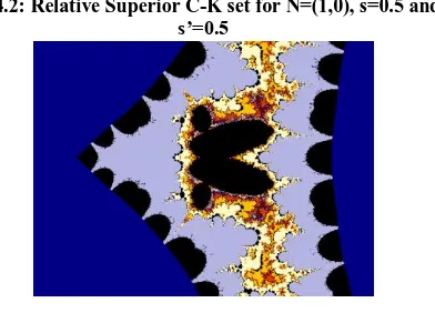
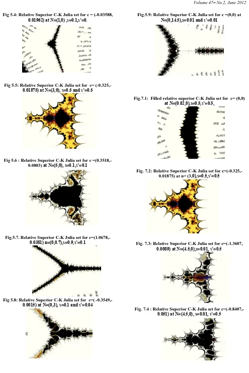
Fig 5.4: Relative Superior C-K Julia set for c = (-0.03588, 0.01962) at N=(1,0) ,s=0.1,s’=0.
Fig 5.5: Relative Superior C-K Julia set for c= (-0.325,-0.01875) at N=(3,0), s=0.5 and s’=0.5
Fig 5.6 : Relative Superior C-K Julia set for c =(0.3518,-0.0803) at N=(5,0), s=0.1,s’=0.1
Fig.5.7. Relative Superior C-K Julia set for c=(1.0678,-0.0381) n=(0,0.7),s=0.9,s’=0.1
Fig 5.8: Relative Superior C-K Julia set for c=( -0.3549,-0.0015) at N=(0,3), s=0.1 and s’=0.04
Fig.5.9: Relative Superior C-K Julia set for c =(0,0) at N=(0,14.5),s=0.01 and s’=0.01
Fig.7.1: Filled relative superior C-K Julia set for c= (0,0) at N=(0.02,0),s=0.5,s’=0.5,
Fig. 7.2: Relative Superior C-K Julia set for c=(-0.325,-0.01875) at n= (3,0),s=0.5,s’=0.5
Fig. 7.3: Relative Superior C-K Julia set for c=(-1.3607, 0.0089) at N=(4.5,0),s=0.01, s’=0.5
Fig 7.5: Relative Superior C-K Julia set for N=(5.5,0),s=0.05,s’=0.04,c=(0.3492,0.0875)
Fig.7.6: Relative Superior C-K Julia for N= (9.5, 0), s = 0.09, s’=0.1,c = (0, 0)
Fig.7.7: Relative Superior C-K Julia set for c=(-0.09,0.1) at n= (9.5,0) s=0.01,s’=0.5
Fig.7.8: Zoom of portion of Superior Julia set for N=(0,0.2), s=0.1,s’=0.01 C=(0,0)
[image:5.595.73.534.36.806.2]Fig.7.9: Relative Superior C-K Julia set for c =(-0.7374,0.0009) at N=(0,4.5), s=0.0,1s’=0.5
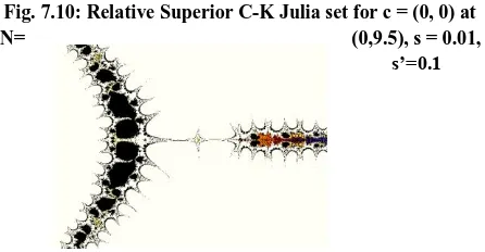
Fig. 7.10: Relative Superior C-K Julia set for c = (0, 0) at
N= (0,9.5), s = 0.01,
s’=0.1
Fig. 7.11: Relative Superior C-K Julia set for c=(1.0678,-0.0381) at N =(0,0.7), s=0.9, s’=0.1
Fig. 7.12: Part of Relative Superior C-K Julia set for N= (1, 0), s = 0.6, s’=0.5,c = (0, 0)
Fig. 7.13: Part of Relative Superior C-K Julia set for N= (1, 0), s = 1, s’=0.5,c = (0, 0) rotated 90 degrees.
6.
FIXED POINTS
[image:5.595.318.541.72.188.2]Table 6.1.1: Orbit of F(z) for c=(0,0) at N=(0.02,0), s=0.5 and s’=0.5
[image:6.595.354.500.139.256.2] [image:6.595.341.519.293.486.2] [image:6.595.93.248.313.438.2] [image:6.595.350.512.526.689.2]No. of Iteration
|F(z)| No. of Iteration
|F(z)|
1. 0.0000 16. 2.8528
2. 1.4614 17. 2.8528
3. 2.1883 18. 2.8528
4. 2.5381 19. 2.8528
5. 2.7046 20. 2.8528
6. 2.7836 21. 2.8528
7. 2.8208 22. 2.8528
8. 2.8382 23. 2.8528
9. 2.8462 24. 2.8528
10. 2.8499 25. 2.8528
11. 2.8515 26. 2.8528
12. 2.8523 27. 2.8528
13. 2.8526 28. 2.8528
14. 2.8527 29. 2.8528
15. 2.8528 30. 2.8528
Fig. 6.1.1: Orbit of F(z) for c=(0,0) at real( N)=0.02 and
s=0.5 and s’=0.5
Table 6.1.2: Orbit of F(z) for c=(-0.0359,0.01962) at N=(1,0) and s=0.5, s’=0.5
No. of Iteration
|F(z)| No. of Iteration
|F(z)|
1. 0.0000 16. 0.7935
2. 0.4020 17. 0.7936
3. 0.5894 18. 0.7936
4. 0.6826 19. 0.7936
5. 0.7316 20. 0.7936
6. 0.7584 21. 0.7936
7. 0.7735 22. 0.7936
8. 0.7822 23. 0.7936
9. 0.7872 24. 0.7936
10. 0.7900 25. 0.7936
11. 0.7916 26. 0.7936
12. 0.7925 27. 0.7936
13. 0.7930 28. 0.7936
14. 0.7933 29. 0.7936
15. 30.
16. 0.7935 31. 0.7936
Fig. 6.1.2: Orbit of F(z) for c=(-0.0359,0.01962) at N=(1,0) and s=0.5,s’=0.5
Table 6.1.3: Orbit of F(z) for c= =(-0.325,-0.01875) at (N=3,0) and s=0.5, s’=0.5
Here the value converges after 16 iterations
No. of Iteration
|F(z)| No. of Iteration
|F(z)|
1. 0.0000 16. 0.0669
2. 0.0475 17. 0.0668
3. 0.0563 18. 0.0668
4. 0.0609 19. 0.0668
5. 0.0635 20. 0.0668
6. 0.0650 21. 0.0668
7. 0.0659 22. 0.0668
8. 0.0665 23. 0.0668
9. 0.0668 24. 0.0668
10. 0.0669 25. 0.0668
11. 0.0670 26. 0.0668
12. 0.0670 27. 0.0668
13. 0.0669 28. 0.0668
14. 0.0669 29. 0.0668
15. 0.0669 30. 0.0668
Table 6.1.4 : Orbit of F(z) for c= =(0.3518,-0.0803) at N=(5,0) and s=0.1,s’=0.1
[image:7.595.342.514.114.245.2]Here the value converges after 10 iterations
Fig. 6.1.4 : Orbit of F(z) for c= =(0.3518,-0.0803) at N=(5,0) and s=0.1,s’=0.1
[image:7.595.335.524.295.485.2]6.2
Fixed points when real N = 0
Table.6.2.1: Orbit of F(z) for , c= (1.067813364,-0.038102687) at N=(0, 0.7), s=0.9, s’=0.1
[image:7.595.71.262.534.722.2] [image:7.595.355.486.651.771.2]No. of Iteration
|F(z)| No. of Iteration
|F(z)|
1. 0.0000 16. 1.5670
2. 1.8726 17. 0.3831
3. 0.3564 18. 1.5670
4. 1.5981 19. 0.3831
5. 0.3737 20. 1.5670
6. 1.5777 21. 0.3831
7. 0.3797 22. 1.5670
8. 1.5708 23. 0.3831
9. 0.3819 24. 1.5670
10. 1.5684 25. 0.3831
11. 0.3827 26. 1.5670
12. 1.5675 27. 0.3831
13. 0.3830 28. 1.5670
14. 1.5672 29. 0.3831
15. 0.3831 30. 1.5670
Here we get two fixed points after 15 iterations
Fig. 6.2.1: Orbit of F(z) for , c= (1.067813364,-0.038102687) at N=(0, 0.7), s=0.9, s’=0.1
Table.6.2.2Orbit of F(z) for c=( -0.3549,-0.0015) at N=(0,3), s=0.1, s’=0.04
No. of Iteration
|F(z)| No. of Iteration
|F(z)|
1. 0.0000 16. 0.0908
2. 0.0481 17. 0.0996
3. 0.0138 18. 0.0908
4. 0.0602 19. 0.0996
5. 0.0349 20. 0.0908
6. 0.0742 21. 0.0996
7. 0.0625 22. 0.0908
8. 0.0858 23. 0.0996
9. 0.0879 24. 0.0908
10. 0.0904 25. 0.0996
11. 0.0987 26. 0.0908
12. 0.0909 27. 0.0996
13. 0.0997 28. 0.0908
14. 0.0908 29. 0.0996
15. 0.0996 30. 0.0908
Here we get two fixed points after 14 iterations
Fig 6.2.2 Orbit of F(z) for c=( -0.3549,-0.0015) at N=(0,3), s=0.1,s’=0.04
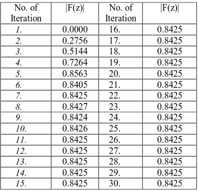
No. of Iteration
|F(z)| No. of Iteration
|F(z)|
1. 0.0000 16. 0.8425
2. 0.2756 17. 0.8425
3. 0.5144 18. 0.8425
4. 0.7264 19. 0.8425
5. 0.8563 20. 0.8425
6. 0.8405 21. 0.8425
7. 0.8425 22. 0.8425
8. 0.8427 23. 0.8425
9. 0.8424 24. 0.8425
10. 0.8426 25. 0.8425
11. 0.8425 26. 0.8425
12. 0.8425 27. 0.8425
13. 0.8425 28. 0.8425
14. 0.8425 29. 0.8425
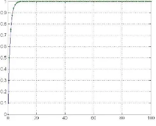
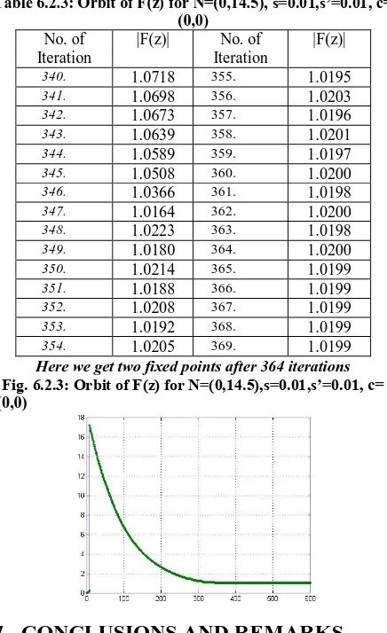
Table 6.2.3: Orbit of F(z) for N=(0,14.5), s=0.01,s’=0.01, c= (0,0)
No. of Iteration
|F(z)| No. of Iteration
|F(z)|
340. 1.0718 355. 1.0195
341. 1.0698 356. 1.0203
342. 1.0673 357. 1.0196
343. 1.0639 358. 1.0201
344. 1.0589 359. 1.0197
345. 1.0508 360. 1.0200
346. 1.0366 361. 1.0198
347. 1.0164 362. 1.0200
348. 1.0223 363. 1.0198
349. 1.0180 364. 1.0200
350. 1.0214 365. 1.0199
351. 1.0188 366. 1.0199
352. 1.0208 367. 1.0199
353. 1.0192 368. 1.0199
354. 1.0205 369. 1.0199
Here we get two fixed points after 364 iterations Fig. 6.2.3: Orbit of F(z) for N=(0,14.5),s=0.01,s’=0.01, c= (0,0)
7.
CONCLUSIONS AND REMARKS
In this paper we studied the Carotid Kundalini function which is one of the members of transcendental family. We generated different Julia set for C-K function using the Relative Superior iterates and studied their characteristics. The fractals and the Julia sets generated shows symmetry along the real axis for both Real and Imaginary values. The relative superior Carotid Kundalini set and its Julia set takes up the shape of < and appears to be an invariant Cantor set in the form of curves or “dendrites “that extends to
. The orbit of any point on the dendrites tends to infinity under iteration. This geometry of the dendrites is quite similar to that of exponential family showing the property of transcendental function.Finally we concluded that for both the real and imaginary values , the repeated iteration of C-K function produced values which exhibited three different types of behaviour, i.e the values either converged to a fixed point, displayed periodic motion or increased indefinitely at each iteration. We get some beautiful images that resemble the Yoga Kundlaini from Hindu Mythology; hence we can say that the name Carotid-Kundalini is justified.
8.
ACKNOWLEDGMENTS
I would like to thanks Mr. Yashwant S. Chauhan and Rajshri Rana, Asst. Professor, G.B.Pant Engineering College, Pauri Garhwal, Uttarakhand for their valuable suggestions .
9.
REFERENCES
[1] Cooper, G.R.J.: Julia sets for complex Carotid-Kundalinifunction, Computers and Graphics 25(2001),153-158.
[2] Cooper, G. R. J.: Chaotic behavior in the Carotid – Kundalini map function, Computer Graphics 2000;24,165-70.
[3] Devaney, R. L.: Chaos, Fractals and dynamics, Computer experiments in mathematics, Menlo Park, Addison – Wessley (1992).
[4] Devaney, R. L.: The fractal Geometry of the Mandelbrot set , 2.How to count and how to add . Symposium in honor of Benoit Mandelbrot (Curaco 1995), Fractal 1995;3(4),629-40[MR1410283(99d:58095)].
[5] Devaney, R. L. and Krych M.: “Dynamics of exp(z)”, Ergodic Theory Dynam. Systems4 (1984), 35–52. [6] Devaney, R. L. and Tangerman F. : “ Dynamics of entire
functions near the essential singularity”, Ergodic Theory and Dynamical Systems 6 4 (1986) 489–503. [7] Devaney, R. L. and Tangerman F.: “Dynamics of
entire functions near the essential Singularity”, Ergodic Theory Dynam. Systems 6 (1986), 489–503. [8] Peitgen, H. O.; Jurgens, H.; Saupe, D.: Chaos and
Fractals, New frontiers of science, New York Springer,1992 984pp.
[9] Eremenko A.: “Iteration of entire functions”, Dynamical Systems and Ergodic theory Banach Center Publ. 23, Polish Sc. Pub. , Warsaw 1989, 339-345.
[10]Pierre Fatou, “ Sur Iteration des functions transcend dantesentires “ Acta Math 47(1926),337-378
[11]Rani, M.; Kumar, V.: Superior Julia set, J Korea Soc Math Edu Series D: Res Math Edu 2004; 8(4), 261-277.
[12]Rani M.: Iterative Procedures in Fractal and Chaos, Ph.D. Thesis, Department of Computer Science, Gurukul Kangri Vishwavidhayalaya, Hardwar,2002.
[13] Julia, G.: Sur 1‟ iteration des functions rationnelles, J Math Pure Appl., 1918; 8, 47-245.
[14]Rottenfußer G. , Schleicher D.: Escaping Points of the Cosine Family, arXiv: math/0403012 (March 2004) [15]McMullen C.: “Area and Hausdorff dimension of
Julia sets of entire functions”, Transactions of the American Mathematical Society 300 1 (1987), 329–342. [16]Ishikawa S.: Fixed points by a new iteration method”,
Proc. Amer. Math. Soc.44 (1974), 147-150.
[17]Rani, Negi A.: Newjulia sets for complex c-k function,
[18]ChauhanS.Y ,RanaR.andNegiA.: “New Julia Sets of Ishikawa Iterates”, International Journal of Computer Applications 7(13):34–42, October 2010. Published By Foundation of Computer Science.ISBN: 978-93-80746-97-5
[19]Rana R.,Yashwant S Chauhan and Negi A.:. “Non Linear Dynamics of Ishikawa Iteration”, International Journal of Computer Applications 7(13):43–49, October 2010. Published By Foundation of Computer Science. ISBN: 978-93-80746-97-5.
[20]Chauhan S. Y.; Rana, R.; Negi, A.; New Tricorn & Multicorns of ishikawa Iterates, International Journal of Computer Applications(0975-8887), Vol 7, No. 13, October 2010.
[21]Rana R.,Chauhan, S. Y. andNegi, A.; Inverse Complex Function Dynamics of Ishikawa Iterates , International Journal of Computer Applications(0975-8887), Vol 9, No. 1, November 2010.
International Journal of Computer Applications(0975-8887), Vol 9, No. 2, November 2010.
[23]Peitgen H. and RichterP. H., The Beauty of Fractals, Springer-Verlag, Berlin,1986.