Design of centralized CRONE controller combined with MIMO QFT approach applied to non square multivariable systems

Design of Centralized CRONE Controller Combined with

MIMO-QFT Approach Applied to Non Square

Multivariable Systems

Najah Yousfi

1

, Pierre Melchior

2

, Chokri Rekik

1

, Nabil Derbel

1

, Alain Oustaloup

2

1 Control & Energy Management laboratory (CEM), University of Sfax, Sfax Engineering School, BP W, 3038 Sfax, Tunisia.

2 IMS (UMR 5218 CNRS, Université Bordeaux 1 - ENSEIRB - ENSCPB), Département LAPS 351 cours de la Libération, Bât. A4 - F33405 TALENCE cedex, France.

ABSTRACT

Motion control and robust path tracking were extended to non square MIMO systems having more outputs then inputs in this work. The Non square Relative Gain array (NRG) has been used to assess the performance of non-square control systems based on steady-state information. Using NRG and the SSE (Sum of Square Error), a square subsystem can be selected. MIMO-QFT (Quantitative Feedback Theory) robust synthesis methodology permits to generate the appropriate equivalent MISO (Multi-input Single-Output) system structure from the MIMO (Multi-Input Multi-Output) structure. After that, the CRONE control approach based on third generation CRONE methodology was used to find the controller of the selected subsystem taking into account plant uncertainties. A fractional prefilter synthesis approach was already developed to find a non-integer prefilter expression in order to satisfy the performance specifications. A fully populated matrix controller structure has been proposed to govern perfectly the multivariable processes. In order to reduce the loop interactions, a coupling matrix has been designed. A numerical example has been treated in order to verify the proposed design.

General Terms

Path tracking design using CRONE control approach applied to non-square multivariable systems.

Keywords

Path tracking, Non square relative gain array (NRG), CRONE control design, Motion control, Coupling effect, Robotics.

1.

INTRODUCTION

Multivariable systems with uncertainty can be considered one of the hardest problems in industry because most of complex industrial processes are always Multi-Input Multi- Output (MIMO) systems. MIMO systems are more difficult to control due to the existence of interactions among input and output variables.

Several researches have been used in robust generation and path tracking design. In industrial path tracking designs, a prefilter is used since it is easy to implement and adapt to reduce overshoots. One of most used prefilter is that of Davidson-Cole whose main property is eliminating overshoots on the plant output. It is possible by using the Davidson-Cole filter to limit the resonance of the feedback control loop, by a continuous variation on its two constitutive parameters time constant _ and real order n. A MIMO-QFT robust synthesis methodology has been used by Melchior [1] which is applied to a square MIMO system in path tracking design. The general problem in the QFT Two Degree Of Freedom (TDOF) system is how to generate the feedback controller and the prefilter [2]. Specifications of most QFT problems are to put the responses of the closed loop system into lower and upper bounds [2], [3], [4], [5], [6].

Nevertheless, the original MIMO-QFT design usually proposes the use of diagonal controller to control multivariable systems. A non-diagonal controller has been used to improve this structure. More design flexibility in the control of MIMO plants can be given by the non diagonal controller. Other alternative methods for non-diagonal multivariable QFT robust control system design have been introduced [7]. Garsia sanz et al. [8], [9], [10] extends the classic QFT diagonal controller design for square MIMO plants with uncertainty to a fully populated matrix controller structure. The QFT approach can be combined with different type of controller like CRONE control approach which is the aim of this work.

The CRONE control-system design is initially introduced by Oustaloup et al. [11], [12]. This methodology is based on fractional non-integer differentiation [13], [14]. The Crone control is a frequency design to provide the robust control of perturbed plants using the common unity feedback con- figuration. For the nominal state of the plant, this approach consists in determining the open-loop transfer function which guarantees the desired specifications like precision, overshoot and rapidity. The controller can be obtained from the ratio of the open loop transfer function to the nominal plant transfer function taking into account the plant right half-plane zeros and poles. There are three CRONE control generations [15], [16]. Only the used principle of the third generation is given in this paper.

The fractional non-integer differentiation allows to describe the open-loop transfer function. The optimal transfer function to meet the specifications is easier to obtain. Furthermore, the CRONE control design takes into account the plant genuine structured uncertainty domains. CRONE control design has already been applied to multivariable systems [15], [17]. Usually square MIMO systems are used in industry process. These type of systems have got an equal number of inputs and outputs. Yet, when one of actionnera is nonfunctional then the studied system become having more outputs than inputs. This paper resolves the problem of non square MIMO system which has more outputs than inputs in path tracking design. So, the aim of this work is to extend the CRONE control approach to non square MIMO systems using fractional prefilters in path tracking design. A combined CRONE control and MIMO-QFT structure using non diagonal controller have been developed to compare the utility of using fractional prefilter. The non square relative gain array (NRG) [18] is a useful tool to analyze a non square multivariable systems. NRG is used to determine the interaction measurements. This approach can help to square down the non square multivariable systems.

methodology for multivariable plants. A fractional prefilter optimization is given in section 5. Finally, an example is employed to illustrate the effectiveness of the proposed methodology to control non square multivariable system in section 6.

2.

CONTROL STRUCTURE FOR

NON-SQUARE MULTIVARIABLE SYSTEMS

2.1

Non-square relative gain array (NRG)

Consider a 𝑚 × 𝑛 process transfer function 𝑃with m ≥ n :

𝑃 𝑝 =

𝑝

₁₁

⋯ 𝑝

_1𝑛

⋮

⋱

⋮

𝑝

_𝑚1

⋯ 𝑝

_𝑚𝑛

(1)

The non-square relative gain array is a way to measure interaction between inputs and outputs. The non-square relative gain array can be evaluated:

𝛬𝑁 _{𝑝 = 𝑃 ⊗ 𝑃}∗ 𝑇 ₍₂₎ where the operator ⊗ is the Hadamard product and P∗ represent the Moore-Penrose Pseudo-inverse transfer matrix of P.

𝛬𝑁 𝑝 =

𝜆𝑁

11 ⋯ 𝜆𝑁1𝑛

⋮ ⋱ ⋮

𝜆𝑁

𝑚1 ⋯ 𝜆𝑁𝑚𝑛

(3)

The sum of all elements in each row 𝑅𝑆 and in each column

𝑅𝐶 is defined as:

𝑅𝑆 = 𝑛𝑗 =1𝜆𝑁1𝑗, 𝑛𝑗 =1𝜆𝑁2𝑗, … , 𝑛𝑗 =1𝜆𝑁𝑚𝑗 𝑇

(4) = 𝑟𝑠 1 , 𝑟𝑠 2 , … , 𝑟𝑠(𝑚) 𝑇 (5) rs(i) is the sum of the ith row of the NRG.

and

𝐶𝑆 = 𝑛𝑖=1𝜆𝑁𝑖1, 𝑛𝑖=1𝜆𝑁𝑖𝑗, … , 𝑛𝑗 =1𝜆𝑁𝑚𝑗 𝑇

(6) = 𝑟𝑠 1 , 𝑟𝑠 2 , … , 𝑟𝑠(𝑚) 𝑇 (7) Some properties of non-square multivariable gain array (NRG) have been described by CHANG [18]:

 Sum of elements in each column of the NRG is equal to unity.

𝑐𝑠 𝑗 = 1, ∀ 𝑗

 Sum of elements in each row of the NRG is between zero and unity.

0 ≤ 𝑟𝑠 𝑖 ≤ 1, ∀ 𝑖

 The NRG is invariant under input scaling and variant under output scaling.

 Any permutation of rows and columns in a transfer function matrix P results in the same permutation in the NRG.

 For an m × 1 system, P = [p11; p21,…, pm1]T , so the NRG is described as follow :

𝛬𝑁_{= 𝜆}

11, 𝜆12, … , 𝜆𝑚1𝑇 with

𝛬𝑁

𝑖1= 𝑝𝑖1 2

𝑝𝑘12 𝑚 𝑘=1

 The elements of the NRG approach infinity as the non-square system matrix P becomes nearly singular.

2.2

Control structure selection

CHANG [18] was used an approach to design a control system for a non-square process. This approach help to square down the non-square system. Consider a non-square plant, P. It can be partitioned into a square subsystem Ps and a complementary (remaining) subsystem Pr. The control objective is to minimize the sum of square error (SSE) of uncontrolled outputs when the square subsystem is under perfect control. The row sum of the NRG (Non-square Relative Gain array) provides some information in this regard. For an

m× n

process with

m > n

, if we choose n outputs for control the system can be partitioned into (see Figure 1):

Fig 1 Control structure for TDOF MIMO system

then

𝑦𝑠 − 𝑦𝑟

= 𝑃−𝑠 𝑃𝑟

. 𝑢 =

𝑝_.11 . 𝑝1𝑛

𝑝_𝑛1 . 𝑝𝑛𝑛

− − −

𝑝𝑚1 . 𝑝𝑚𝑛

. 𝑢

(8)

where 𝑦𝑠is an n × 1 output vector for the controlled outputs and 𝑦𝑟 is an m−n ×1 output vector for the remaining output. The objective is to minimize the Sum of Square Error (SSE) of the uncontrolled outputs for any variation in the controlled outputs.

The closed loop square subsystem gains are given by:

𝑢 = 𝑃

𝑠−1𝑦 𝑠𝑠𝑒𝑡 (9) For all outputs, the steady state error is:

𝑒 = (𝐼𝑚×𝑛− 𝑃𝑃𝑠−1)𝑦 𝑠𝑠𝑒𝑡 (10) Choosing a particular square subsystem, 𝑃𝑠, the SSE is defined as:

𝑆𝑆𝐸 = 𝑛𝑖=1 𝑒 (𝑖) 22= 𝑛𝑖=1 (𝐼𝑚×𝑛− 𝑃𝑃𝑠−1)𝑦 𝑠𝑒𝑡𝑠,𝑖 2 2

(11) The row sum of NRG provides optimal solution to the

problem for two special cases, namely, case of n = 1 and case of m = n + 1, and suboptimal solution of other cases [18].

2.2.1

Case of

𝑚 = 𝑛 + 1

A square subsystem is chosen, the sum of square error is given by:

𝑆𝑆𝐸 =_{1−𝑟𝑠(𝑛+2−𝑗 )}𝑟𝑠(𝑛+2−𝑗 ) (12) where j means the sum of square error when the jth _{subset is} chosen to form a square subsystem.

3.

CENTRALIZED CONTROLLER

3.1

Coupling matrix

QFT approach has been developed to control MIMO systems. This approach, usually, uses diagonal controller. Whereas MIMO QFT procedures take into account the coupling effect between loops. They only use a diagonal controller G to govern the MIMO plant. This method has been improved using non-diagonal controllers [8], [9], [10]. Most design flexibility in the control of MIMO plants was given using a fully populated matrix. Also, the non-diagonal components can simply the diagonal controller design problem.

A measurement index has been defined in order to quantify the loop interactions in MIMO control systems.

[image:3.595.47.547.61.806.2]

The MIMO-QFT structure is given by figure 2. This figure is composed of a 𝑛 × 𝑛 multivariable uncertain plant 𝑃𝑠, a fully populated matrix controller 𝐺 and a prefilter 𝐹.

Fig 2 Two-degrees-of-freedom control system: MIMO structure

 𝑃𝑠 𝑝 is n × n transfer function matrix. 𝑃𝑠 represents a linear time invariant uncertain and minimum-phase plant. The plant 𝑃𝑠 and its inverse 𝑃𝑠∗ must be stable and having no unstable modes. 𝑃𝑠 ∈⟧𝑃𝑠 where ⟧𝑃𝑠 is a

set of possible uncertain plants. 𝑃 𝑝 =

𝑝11(𝑝) ⋯ 𝑝1𝑛(𝑝)

⋮ ⋱ ⋮

𝑝𝑛1(𝑝) ⋯ 𝑝𝑛𝑛(𝑝)

(13)

 𝐺(𝑝) is the non-diagonal controller

𝐺 𝑝 =

𝑔11(𝑝) ⋯ 𝑔1𝑛(𝑝)

⋮ ⋱ ⋮

𝑔𝑛1(𝑝) ⋯ 𝑔𝑛𝑛(𝑝)

(14)

 𝐹(𝑝) is the non-diagonal controller

𝐹 𝑝 =

𝑓11(𝑝) ⋯ 𝑓1𝑛(𝑝)

⋮ ⋱ ⋮

𝑓𝑛1(𝑝) ⋯ 𝑓𝑛𝑛(𝑝)

(15)

The plant inverse is denoted 𝑃𝑠∗so:

𝑃𝑠−1 𝑝 = 𝑃𝑠∗ 𝑝 = 𝑝𝑖𝑗∗(𝑝) = 𝛬 𝑝 + 𝐵 𝑝 (16) where:

𝛬 𝑝 =

𝑝11∗ (𝑝) ⋯ 0

⋮ ⋱ ⋮

0 ⋯ 𝑝𝑛𝑛∗ (𝑝)

and

𝐵 𝑝 = 0 ⋯ 𝑝1𝑛

∗ _(𝑝)

⋮ ⋱ ⋮

𝑝𝑛1∗ (𝑝) ⋯ 0

Elements 𝑞𝑖𝑗 of matrix 𝑄 are described by:

𝑞𝑖𝑗 𝑝 =_𝑝 1

𝑖𝑗∗(𝑝) (17)

The controller, 𝐺(𝑝), is divided to this form:

𝐺 𝑝 = 𝐺𝑑 𝑝 + 𝐺𝑏(𝑝) (18) where

𝐺𝑑 𝑝 =

𝑔11(𝑝) ⋯ 0

⋮ ⋱ ⋮

0 ⋯ 𝑔𝑛𝑛(𝑝)

and

𝐺𝑏 𝑝 =

0 ⋯ 𝑔1𝑛(𝑝)

⋮ ⋱ ⋮

𝑔𝑛1(𝑝) ⋯ 0

𝛬 and 𝐺𝑑are respectively the diagonal part of 𝑃 𝑝 and 𝐺(𝑝), wheras 𝐵 is the balance of 𝑃𝑠∗ and 𝐺𝑑is the balance of 𝐺. The controlled system for the reference tracking problem can be written as:

The controlled system for the reference tracking problem, can be written as:

𝑦𝑠= 𝐼 + 𝑃𝑠𝐺 −1𝑃𝑠𝐺𝑟 (19) = 𝑇𝑦𝑠/𝑟𝐹𝑟′

(19) can be reformulated using (16) and (18):

𝑇𝑦𝑠/𝑟𝑟 = 𝐼 + 𝛬

−1_𝐺

𝑑 −1𝛬−1𝐺𝑑𝑟 + (20) 𝐼 + 𝛬−1𝐺𝑑 −1𝛬−1 𝐺𝑏𝑟 − 𝐵 + 𝐺𝑏 𝑇𝑦𝑠/𝑟𝑟

Observing the expression of the closed-loop transfer function matrix (20), two different terms can be found which are the diagonal 𝑇𝑦𝑠/𝑟−𝑑and the non diagonal 𝑇𝑦𝑠/𝑟−𝑏 terms.

𝑇𝑦𝑠/𝑟−𝑑= 𝐼 + 𝛬

−1_𝐺

𝑑 −1𝛬−1𝐺𝑑 (21)

𝑇𝑦𝑠/𝑟−𝑏= 𝐼 + 𝛬

−1_𝐺

𝑑 −1𝛬−1 𝐺𝑏− 𝐵 + 𝐺𝑏 𝑇𝑦𝑠/𝑟

= 𝐼 + 𝛬−1𝐺𝑑 −1𝛬−1𝐶 (22)

The only part that related to the non-diagonal terms of both plant inverse B and controller Gb is the matrix C. For reference tracking problems, C is called the coupling matrix.

𝐶 = 𝐺𝑏− 𝐵 + 𝐺𝑏 𝑇𝑦𝑠/𝑟 (23)

Each elements of this matrix respect:

𝑐𝑖𝑗= 𝑔𝑖𝑗 1 − 𝛿𝑖𝑗 − 𝑛𝑘=1 𝑝𝑖𝑘∗ + 𝑔𝑖𝑘 𝑡𝑘𝑗 1 − 𝛿𝑖𝑗 (24)

(21) is equivalent to n reference tracking single-input single- output where plants are equal to the elements of 𝛬−1 and (22) is equivalent to the same n previous systems with internal disturbances 𝑐𝑖𝑗𝑟𝑗. So, the ith MISO structure is as follow:

Fig 3 ith equivalent MISO system

To analyse the coupling element, Garsia-Sanz [8], [9] supposes that∀ 𝑘 ≠ 𝑗, |𝑡𝑗𝑗 𝑝𝑖𝑗∗ + 𝑔𝑖𝑗 | ≫ |𝑡𝑘𝑗 𝑝𝑖𝑘∗ + 𝑔𝑖𝑘 |. This assumption leads to two simplifications which facilitate the coupling expression:

1. S1 𝑐𝑖𝑗 = 𝑔𝑖𝑗− 𝑡𝑗𝑗 𝑝𝑖𝑗∗ + 𝑔𝑖𝑗 ; 𝑖 ≠ 𝑗 2. S2 𝑡𝑗𝑗 =

𝑔𝑗𝑗𝑞𝑗𝑗

1+𝑔𝑗𝑗𝑞𝑗𝑗

The coupling effects 𝑐𝑖𝑗 using S1 and S2 becomes: 𝑐𝑖𝑗= 𝑔𝑖𝑗−

𝑔𝑗𝑗 𝑝𝑖𝑗∗+𝑔𝑖𝑗

𝑝_𝑗𝑗∗_+𝑔

3.2

Controller design

The optimum non diagonal controller is found making the coupling effect (25) equal to zero.

𝑔_𝑖𝑗𝑜𝑝𝑡 = 𝐹𝑝𝑑 𝑔𝑗𝑗 𝑝𝑖𝑗∗𝑁

𝑝_𝑗𝑗∗𝑁 , 𝑖 ≠ 𝑗 (26)

The proposed controller is deduced from a sequential procedure. The first step is pairing outputs and inputs using RGA methods. The sequential controller approach composed of n stages which is the number of loops. The second step is the design of the diagonal controller 𝑔𝑘𝑘. The controller 𝑔𝑘𝑘is calculated using the CRONE control approach [12], [14] for the inverse of the equivalent plant 𝑝𝑘𝑘∗𝑒(𝑝) 𝑘−1so that obtaining robust stability and robust performance specifications. The equivalent plant is introduced by Horowitz [7] and ameliorated by Franchek et al [19].

𝑝𝑖𝑗∗𝑒 𝑝 _𝑘 =

𝑝𝑖𝑗∗𝑒 𝑝 _𝑘−1−

𝑝_{𝑖 𝑘−1} ∗𝑒 _𝑝

𝑘−1+ 𝑔𝑖 𝑘−1 𝑝 𝑘−1

𝑝 _{𝑘−1 𝑘−1} ∗𝑒 _𝑝

𝑘−1+ 𝑔 𝑘−1 𝑘−1 𝑝 𝑘−1

(27)

× 𝑝 _{𝑘−1 𝑗}∗𝑒 _𝑝

𝑘−1+ 𝑔 𝑘−1 𝑗 𝑝 𝑘−1

After that, the non diagonal part of the controller is designed to minimize the coupling effects (see(26)).

Finally, a fractional prefilter F is determined which does not present any difficulty to make the closed loop transfer function into the desired specifications.

4.

CRONE CONTROL

The CRONE control approach is a frequential approach based on fractional derivative. The object of this method is how to design a controller which allows a degree of stability robustness. There are three generations describing the control law. In this paper we will focus on the third generation CRONE control because the plant frequency uncertainty domains are of various types. The third-generation CRONE can manage the robustness/performance tradeoff. Also, it is able to synthesis controllers for plants with positive real part zeros or poles, with lightly damped mode, and/or time delay [20]. For multivariable plant (MIMO) two methods have been developed [21], multivariable and multi-SISO approach. The objective is to succeed output feedback decoupling. Therefore, the decoupling and diagonal open-loop transfer matrix will allow a diagonal nominal closed-loop transfer matrix:

𝛽0 𝑝 =

𝛽01(𝑝) … … 0

0 ⋱ … …

… … 𝛽0𝑖(𝑝) 0

0 … 0 𝛽0𝑛(𝑝)

(28)

The nominal sensitivity 𝑆0(𝑝), the nominal complementary sensitivity 𝑇0(𝑝), input sensitivity 𝑆𝑈0(𝑝) and input disturbance sensitivity 𝑆𝑙0(𝑝), transfer function matrices are:

𝑆0 𝑝 = 𝐼 + 𝛽0 𝑝 −1= 𝑑𝑖𝑎𝑔 𝑆0𝑗 𝑝 _{1≤𝑗 ≤𝑛} (29)

𝑇0 𝑝 = 𝐼 + 𝛽0 𝑝 −1𝛽0 𝑝 = 𝑑𝑖𝑎𝑔 𝑇0𝑗 𝑝 _{1≤𝑗 ≤𝑛} (30)

𝑆𝑈0 𝑝 = 𝐺(𝑝) 𝐼 + 𝛽0 𝑝 −1= 𝐺(𝑝) 𝑆0 𝑝 (31)

𝑆𝑙0 𝑝 = 𝐼 + 𝛽0 𝑝 −1𝑄(𝑝) = 𝑇0 𝑝 𝐺−1(𝑝) (32)

With:

𝑇

_0𝑗

𝑝 =

𝛽0 𝑝

1+𝛽0 𝑝

(33)

𝑆

0𝑗

𝑝 =

_1+𝛽1

0 𝑝

(34) The open-loop transfer functions 𝛽0𝑖 𝑝 are used to satisfy some objectives:

 accuracy specifications at low frequencies,

 required nominal stability margins of the closed-loops

 specifications on the n control efforts at high frequencies.

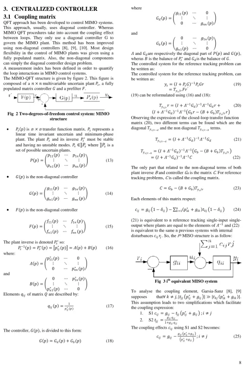
[image:4.595.333.523.266.421.2]

The third generation of CRONE CSD uses complex non integer order integration over a selected frequency range [ωA, ωB]. The generalized template is a straight line of any direction in the Nichols chart created by the complex fractional order nf = a + ib (figure 4):

Fig 4 The generalized template

Its phase location at frequency 𝜔𝑐𝑔 is given by the real part of

𝑛𝑓 and the imaginary part defines its direction [22]. When the generalized template is based on band-limited complex non-integer integration, then the transfer function is [23], [24]:

𝛽0𝑖 𝑝 = 𝐶𝑠𝑖𝑔𝑛 (𝑏)

1 + 𝑝/𝜔𝑕

1 + 𝑝/𝜔𝑙 𝑎

× 𝑅𝑒/𝑖 𝐶𝑔

1 + 𝑝/𝜔𝑕

1 + 𝑝/𝜔𝑙 𝑖𝑏

−𝑞𝑠𝑖𝑔𝑛 (𝑏)

(35) 𝐶 = 𝑐𝑕 𝑏 𝑎𝑟𝑐𝑡𝑎𝑛 𝜔_𝜔𝑐𝑔

𝑙 −

𝜔𝑐𝑔

𝜔𝑕 (36)

𝐶𝑔= 1+ 𝜔 𝑐𝑔

𝜔 𝑙 2

1+ 𝜔 𝑐𝑔

𝜔 𝑕 2

1/2

(37)

The corner frequencies are placed such that:

𝜔𝑙< 𝜔𝐴< 𝜔𝑐𝑔 < 𝜔𝐵< 𝜔𝑕 (38)

In the open-loop transfer function, the generalized template is taken into account when the plant is stable and minimum phase:

𝛽0𝑖𝑖 𝑝 = 𝛽𝑙𝑖 𝑝 𝛽0𝑖 𝑝 𝛽𝑕𝑖 𝑝 (39) where

𝛽𝑙𝑖 𝑝 = 𝐶𝑙𝑖 𝜔_𝑝𝑙𝑖− 1 𝑛𝑙𝑖

𝛽𝑕𝑖 𝑝 = _𝑝𝐶𝑙𝑖

𝜔 𝑕𝑖+1

𝑛 𝑕𝑖 (41)

The accuracy of each closed-loop is fixed by the order nli but the order nhi allows the elements of the controller to be proper. Consider that Q0 is the nominal plant transfer matrix such that 𝑄0 𝑝 = 𝑞0𝑖𝑗(𝑝) _{𝑖,𝑗 ∈𝑁}: 𝛽0= 𝑄0𝐺 = 𝑑𝑖𝑎𝑔 𝛽0𝑖 𝑖=𝑗 = 𝑑𝑖𝑎𝑔 𝑛_𝑑𝑖 𝑖 𝑖∈𝑁 (42)

where: 𝛽0𝑖=𝑛_𝑑𝑖 𝑖 the element of the i th column and row. The objective of CRONE control for MIMO plants is to determine a decoupling controller for the nominal plant. Q0 being not diagonal, the problem is to find a decoupling and stabilizing controller G. The controller exists if the following hypotheses are true [23]: 𝐻1: 𝑄(𝑝) −1 exists, (43)

𝐻2: 𝑍+[𝑄 𝑝 ] ∩𝑃+ 𝑄 𝑝 = 0 (44)

where 𝑍+[𝑄 𝑝 ] and 𝑃+[𝑄 𝑝 ] are respectively the positive real part zero and pole sets. The controller G is described by: 𝐺 𝑝 = 𝑄0−1 𝑝 𝛽0(𝑝) (45)

For each nominal open-loop 𝛽0(𝑝), many generalized templates can border the same required magnitude-contour of the Nichols chart or the same resonant peak Mp0i. The optimal one minimizes the robustness cost function: 𝐽 = 𝑛𝑖=1 𝑀𝑝_{𝑚𝑎𝑥 𝑖}− 𝑀𝑝_{𝑚𝑖𝑛 𝑖} (46)

where: 𝑀𝑝_{𝑚𝑎𝑥 𝑖}= max𝑄sup𝜔 𝑇𝑖𝑖 𝑗𝜔 (47)

= max𝑄sup𝜔 _1+𝛽𝛽𝑖𝑖(𝑗𝜔 ) 𝑖𝑖(𝑗𝜔 ) 𝑀𝑝_{𝑚𝑖𝑛 𝑖}= min𝑄sup𝜔 𝑇𝑖𝑖 𝑗𝜔 (48)

= min𝑄sup𝜔 _1+𝛽𝛽𝑖𝑖 𝑗𝜔 𝑖𝑖 𝑗𝜔 This optimization can be done while respecting the following set for 𝜔𝜖𝑅 and 𝑖, 𝑗𝜖𝑁 : inf𝑄 𝑇𝑖𝑗 𝑗𝜔 ≥ 𝑇𝑖𝑗𝑙 𝜔 (49)

sup𝑄 𝑇𝑖𝑗 𝑗𝜔 ≥ 𝑇𝑖𝑗𝑢 𝜔 (50)

sup𝑄 𝑆𝑖𝑗 𝑗𝜔 ≥ 𝑆𝑖𝑗𝑢 𝜔 (51)

sup𝑄 𝐺𝑆𝑖𝑗 𝑗𝜔 ≥ 𝐺 𝑆𝑖𝑗𝑢 𝜔 (52)

sup𝑄 𝑆𝑖𝑗 𝑗𝜔 ≥ 𝑆𝑄𝑖𝑗𝑢 𝜔 (53)

where Q is the nominal or perturbed plant. A non-linear optimization method permits the extraction of the independent parameters of each open loop transfer function. Respecting other specifications taken into account by constraints on sensitivity function magnitude, this optimization is based on minimization of the stability degree variations.

5.

FRACTIONAL PREFILTER

OPTIMIZATION

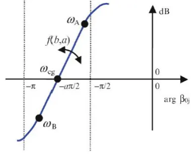
A Davidson-Cole (DC) filter is described by the following transmittance: 𝐹 𝑝 = 1 1+𝜏𝑝 𝑛= 1 1+𝑝_𝜔 𝑛 (54)

[image:5.595.317.519.312.563.2]

which uses real poles and prevents frequency resonance. The choice of identical poles can lead to the largest possible energy on bandwidth (figure.5 (a)). Davidson-Cole prefilter [25] (see (54)), at high frequencies, reduces energy of the signal. As can be seen in figure.5 (b), it continuously controls the bandwidth (time constant τ) and the selectivity (real order n). As analog or digital filter, it can be used as prefilter to reduce overshoots in position control. Fig 5 (a): Pole assignment for a maximum energy in a given pass band; (b) : Frequency response of the Davidson-Cole filter The reference sensitivity transfer function Sref between control u and input r is given by (figure 6): 𝑆𝑟𝑒𝑓 𝑝 = 𝐹 𝑝 𝐺(𝑝) 1+𝐺 𝑝 𝑄(𝑝) (55)

[image:5.595.320.539.612.673.2]

where 𝛾 =𝑢_𝑒𝑚𝑎𝑥

𝑚𝑎𝑥 , with 𝑢𝑚𝑎𝑥 the maximum static constraint

value on the control signal and 𝑒𝑚𝑎𝑥is a constant signal to apply on the prefilter input.

The desired range of the closed-loop transfer function is described by two bounds in frequency domain which are detailed bellow:

∀ 𝜔 > 0, 𝜏 > 0, 𝑇𝑅𝐿 𝑗𝜔 ≤ 𝑡𝑟𝑖𝑖 𝑗𝜔 ≤ 𝑇𝑅𝑈 𝑗𝜔 (57)

This equation becomes:

∀ 𝜔 > 0, 𝜏 > 0, 𝑇𝑅𝐿 𝑗𝜔 ≤ 𝑡𝑟𝑖𝑖 𝑗𝜔 𝑚𝑖𝑛 (58)

𝑡𝑟𝑖𝑖 𝑗𝜔 𝑚𝑎𝑥 ≤ 𝑇𝑅𝑈 𝑗𝜔 (59)

with the closed loop transfer function:

𝑡𝑟𝑖𝑖 𝑗𝜔 =𝑓𝑖𝑖_1+𝑔 𝑗𝜔 𝑔𝑖 𝑗𝜔 𝑞𝑖𝑖 𝑗𝜔

𝑖 𝑗𝜔 𝑞𝑖𝑖 𝑗𝜔 (60)

By considering the integral gap criterion, we can obtain the optimized parameters of the Davidson-Cole filter can be obtained. The integral gap analytic expression for step response is:

𝐼𝑒≤ 𝑛𝜏 (61)

For m × m MIMO systems, the integral gap criterion is calculated as MISO sub-system [8], so in the case of

F =diag [fii] (49) becomes:

𝐼𝑒≤ 𝑛1𝜏1+ 𝑛2𝜏2+ ⋯ + 𝑛𝑚𝜏𝑚 (62)

We can find the optimal parameters of (n, 𝜏 ) using the optimization toolbox of MATLAB.

6.

APPLICATION

Considering a 2 × 3 MIMO uncertain system. It’s transfer function matrix P(p) is :

𝑃 𝑝 =

𝑝11 𝑝12 𝑝21 𝑝22 𝑝31 𝑝32

(63)

𝑝𝑖𝑗(𝑝) = 𝑘𝑖𝑗

1+𝐴𝑖𝑗𝑝 (64)

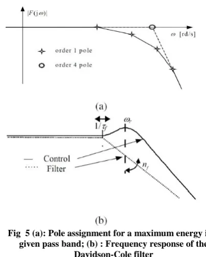
12 cases of plant are given in table 1.

6.1

Pairing rules

From first to fourth plant conditions (table 1), P(0) is :

𝑃 0 = 11 0.52

0.7 5

(65) So, the NRG matrix 𝛬𝑁is described by:

𝛬𝑁=

0.7127 −0.0645

0.4683 −0.0554

−0.1810 1.1199

(66) The sum of elements of each row of 𝛬𝑁 is:

𝑅𝑆 = 0.6482 0.4129 0.9389 𝑇 ₍₆₇₎

Observing RS array (Eq.67), it is clear that the second output which corresponds to the minimum value of RS is the variable that to be eliminated. Then, the rest of 𝛬𝑁becomes𝛬𝑁′:

𝛬𝑁′= 0.7127 −0.0645

−0.1810 1.1199 (68)

According to the NRG matrix 𝛬𝑁′, the paired variables are {u1/y1; u2/y3}. The same technique is used for all other plants.

From five to eight plant cases, the controller structure becomes {u1/y1; u2/y3} and for the rest of plant cases the

variables are paired according to this form {u1/y1; u2/y2}.

Multi-loop controllers are now to be found to control the square subsystem.

6.2

Performance specifications

6.2.1

Tracking specifications

The tracking tolerances must be achieved by |𝑇𝑦/𝑟−𝑑 = 𝑡𝑟𝑖𝑖|(see (57)). The tracking specifications of the closed loop

transfer function are enforced to be into the following upper and lower bounds:

𝑇𝑅𝑈𝑖𝑖 𝑝 =

25 1+0.08𝑝 1+𝑝/25

𝑝2_{+7.5𝑝+25 1+0.002𝑝} (69)

𝑇𝑅𝐿𝑖𝑖 𝑝 =

96

𝑝+1.5 𝑝+8 2 (70)

6.2.2

Controller specifications

The fourth plant is considered as the nominal case. Some specifications must be satisfied for all plant cases:

 For both outputs zero steady-state error

 Settling time as short as possible

 Robustness according to disturbances and parametric variations

 A first overshoot less than 10%.

Some elements of the open-loop transfer matrix can be initialized using these specifications.

6.2.3

Optimization

Respecting all specifications, the initial values for the parameters of the first fractional open-loop transfer function are:

 𝜔𝑟= 5.53434 𝑟𝑎𝑑/𝑠

 𝜔𝑙= 12.0215 𝑟𝑎𝑑/𝑠

 𝜔𝑕 = 242.859 𝑟𝑎𝑑/𝑠

 𝛽01(𝑗𝜔) 𝜔=𝜔_𝑟= 3.07508 𝑑𝐵

 𝑛𝑙= 1

 𝑛𝑕 = 2

And for the second

 𝜔𝑟= 11.0606 𝑟𝑎𝑑/𝑠

 𝜔𝑙= 2.29876 𝑟𝑎𝑑/𝑠

 𝜔𝑕 = 56.7086 𝑟𝑎𝑑/𝑠

 𝛽0₂(𝑗𝜔) _𝜔=𝜔

𝑟= 2.26705 𝑑𝐵

 𝑛𝑙= 1

[image:7.595.140.458.90.384.2]

Table 1 Different conditions of uncertain MIMO systems

N 𝒌𝟏𝟏 𝒌𝟐𝟐 𝒌𝟏𝟐 𝒌𝟐𝟏 𝒌𝟑𝟏 𝒌𝟑𝟐 𝑨𝟏𝟏 𝑨𝟐𝟐 𝑨𝟏𝟐 𝑨𝟐𝟏 𝑨𝟑𝟏 𝑨𝟑𝟐

1 1 2 0.5 1 0.7 5 2 2 4 4.5 2 2

2 1 2 0.5 1 0.7 5 0.5 1 1 3 3 2

3 1 2 0.5 1 0.7 5 0.2 0.4 0.5 2 1.5 2

4 1 2 0.5 1 0.7 5 0.7 0.8 0.3 1 2 2

5 4 5 1 2 3 6 1 2 2 4 4.5 2

6 4 5 1 2 3 6 0.5 1 1 3 3 2

7 4 5 1 2 3 6 0.2 0.4 0.5 2 1.5 3

8 4 5 1 2 3 6 0.7 0.8 0.3 1 2 3

9 10 8 2 4 1 7 1 2 2 4 4.5 3

10 10 8 2 4 1 7 0.5 1 1 3 3 3

11 10 8 2 4 1 7 0.2 0.4 0.5 2 1.5 3

12 10 8 2 4 1 7 0.7 0.8 0.3 1 2 3

Taking into account all specifications, the optimal values for the various parameters of open loop transfer function matrix are:

 For the first loop: 𝐶𝑕1. 𝐶𝑙1= 0.739879, 𝑎1 = 2.02427, 𝑏1= 0.515991, 𝑞1 = 2 and 𝐶1= 1.1006

 For the second loop: 𝐶𝑕2. 𝐶𝑙2= 7.80658, 𝑎2= 1.23807, 𝑏2= −0.511694, 𝑞2= 1 and 𝐶2= 4.82348

6.3

Controller design

Taking into account the desired specifications for the first loop and the model uncertainty of 𝑝11∗ −1, the CRONE control approach is used to find the first loop controller 𝑔11:

𝑔11=1742.7881 𝑝+85.2 𝑝+0.519 _{𝑝 𝑝+380 𝑝+10.4} (71)

Then, minimizing the coupling effect 𝑐21the controller 𝑔21 can be designed (see (26)):

𝑔21=−108.4402 𝑝+0.519 𝑝+0.5 _{𝑝 𝑝+10.4 𝑝+0.2222} (72)

Next, respecting the second loop controller specifications and using the CRONE control approach the controller 𝑔22 for the equivalent plant 𝑃22∗𝑒 −1is calculated:

𝑝22∗𝑒2= 𝑝22∗ 1− 𝑝21

∗

1+ 𝑔211 𝑝12∗ 1+ 𝑔121

𝑝11∗ 1+ 𝑔111 (73)

now, the controller expression is :

𝑔22=365.2146 𝑝+100 𝑝+1.42 𝑝+0.542 𝑝+0.13 _{𝑝 𝑝+90.7 𝑝+21.8 𝑝+1.97 𝑝+0.177} (74)

Finally, the controller 𝑔12 is calculated to minimize the coupling effect:

𝑔12=−91.3037 𝑝+0.542 𝑝+0.13 _{𝑝 𝑝+0.5 𝑝+0.177} (75)

6.4

Prefilter synthesis

The first step consists of selecting the maximum and the minimum plants. The plants number one and eleven are respectively the minimum and the maximum plants. Secondly, the ratio 𝑢_𝑒𝑚𝑎𝑥

𝑚𝑎𝑥 = 1 is fixed. The optimized parameters are

obtained by minimizing the integral gap criterion (61) with

𝑚 = 2 while respecting the frequency bound inequality (55) and the performance specification (56):

𝑛1= 1.0353; 𝜏1= 0.31636 (76) 𝑛2= 1.1273; 𝜏1= 0.405

Using the module “Frequency Domain System Identification” of the CRONE software [26], the integer order approximation of these prefilters is determined :

𝐹 = 𝐹1𝐷𝐶_{0 𝐹}0

2𝐷𝐶 (77) where

𝐹1𝐷𝐶= _{𝑝 + 87.74 𝑝 + 26.61 𝑝 + 3.01} 2.5657 𝑝 + 107 𝑝 + 25.6

𝐹2𝐷𝐶=

0.99433 𝑝 + 539.9 𝑝 + 36.41 𝑝 + 361.1 𝑝 + 25.89 𝑝 + 2.09

𝐹𝑐𝑙= 𝐹𝑐𝑙1_{0 𝐹}0

𝑐𝑙2 (78)

𝐹𝑐𝑙1=_{𝑝 + 2}2

𝐹𝑐𝑙2=_{𝑝 + 1.5}1.5

(a)

(b)

Fig 7 (a),(b) : Closed loop tracking response with classical (red) and fractional prefilters (green), tracking references

(blue)

The closed loop tracking specifications are respected. All plant cases are under upper and lower bounds. The comparison between the two types of prefilters shows the benefit of using fractional prefilters.

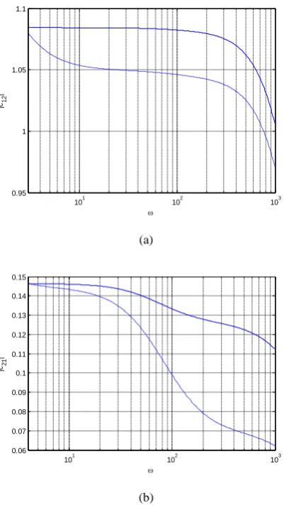
The frequency plot of the obtained coupling reduction for the nominal plant is shown by figure 8.

A significant reduction in the coupling effect using the non diagonal controller is observed. The non diagonal controller is more flexible than the diagonal controller while governing a MIMO system.

(a)

(b) Fig 8 (a) 𝒄_𝟏𝟐𝒈

𝟏𝟐=𝟎 (solid line), 𝒄𝟏𝟐𝒈𝟏𝟐=𝒈𝟏𝟐𝒐𝒑𝒕 (dashed line) and

(b) 𝒄_𝟐𝟏𝒈

𝟐𝟏=𝟎 (solid line), 𝒄𝟐𝟏𝒈𝟐𝟏=𝒈𝟐𝟏𝒐𝒑𝒕 (dashed line)

7.

CONCLUSION

Motion control by fractional prefilter was extended to non-square MIMO systems which is based on MIMO-QFT robust control design combined with CRONE control methodology. In terms of control structure selection, the NRG method has been used. After selection of the square subsystem the CRONE control methodology is used to find the robust controller. The QFT structure uses a non diagonal controller to solve the MIMO reference tracking problem. A coupling matrix has been defined to quantify the amount of loop interaction. The off-diagonal elements of the matrix controller can reduce the cross-coupling. The controller and fractional prefilter have been synthesized in order to put the transfer function of closed loop inside the specified bounds. Both parameters of fractional Davidson-Cole prefilter are optimized on the multiple SISO systems tracking into account the tracking specifications. Validation of this method is applied on a 2x3 MIMO system example.

Thus a prospect is envisaged which concerns the validation of this approach using a real process.

8.

REFERENCES

[1] P. Melchior, C. Inarn, A. Oustaloup. Path tracking design by fractional prefilter extension to square MIMO systems. In Proceedings of the ASME 2009 International Design Engineering Technical Conferences and Computers and Information in Engineering Conference, California, USA, 2009.

0 0.5 1 1.5 2 2.5 3 3.5 4

0 0.2 0.4 0.6 0.8 1 1.2 1.4

Step Response

Time (sec)

A

m

p

lit

u

d

e

0 0.5 1 1.5 2 2.5 3 3.5 4

0 0.2 0.4 0.6 0.8 1 1.2 1.4

Step Response

Time (sec)

A

m

p

lit

u

d

e

101 102 103

0.95 1 1.05 1.1



|c12

|

101 102 103

0.06 0.07 0.08 0.09 0.1 0.11 0.12 0.13 0.14 0.15



|c21

[image:8.595.74.264.49.564.2] [image:8.595.325.526.78.434.2]

[2] S. Mohammad, M. Alavi, A. Khaki Sedigh, B. Labibi, Pre-Filter Design for Tracking Error Specifications in MIMO-QFT, In Proceeding of the 44th IEEE Conference on Decision and Control, and the European Control Conference, Seville, Spain, 2005.

[3] E. Boje, Non-diagonal controllers in MIMO quantitative feedback design, International Journal of Robust and Nonlinear Control, 2002.

[4] W. Zenghui, C. Zengqiang, S. Qinglin, Y. Zhuzh, Multivariable Decoupling Predictive Control Based on QFT Theory and Application in CSTR Chemical Process, Chinese J. Chem. Eng, 2006.

[5] I. Horowitz, Survey of quantitative feedback theory (QFT), International Journal of Robust and Nonlinear Control, 11, 887-921, 2001.

[6] S. Skogestad, I. Postlethwaite, Multivariable feedback control, Analysis and design, Jhon Wiley & Sons, New York, 1996.

[7] I. Horowitz, Improved design technique for uncertain multiple input output feedback systems, International Journal of Control, 36, 977-988, 1982.

[8] M. Garcia-Sanz, I. Egana, Quantitative non-diagonal controller design for multivariable systems with uncertainty, International Journal of Robust and Nonlinear Control, 12, 321-333, 2002.

[9] M. Garcia-Sanz, I. Egana, M. Barreras , Design of quantitative feedback theory non-diagonal controllers for use in uncertain multiple-input multiple-output systems, Control Theory and Applications, IEE Proc., 152, 177-187, 2005.

[10] M. Barreras, C. Villegas, M. Garcia-Sanz, J. Kalkkuhl, “Robust QFT tracking controller design for a Car equipped with 4-Wheel Steer-by- Wire”, Proc. of the 2006 IEEE International Conference on Control Applications, Munich, Germany, October 4-6, 2006. [11] A. Oustaloup, Fractional order sinusoidal oscillators:

optimization and their use in highly linear F.M. modulation, IEEE Transactions on Circuits and Systems, Vol. 28(10), 1007- 1009, 1981.

[12] A. Oustaloup, The CRONE control, In Proceedings of the European Control Conference ECC’91, Grenoble, France, July, 1991.

[13] A. Oustaloup, B. Mathieu, P. Lanusse, Intégration non entière complexe et contours d’isoamortissement, Automatique, Productique, Informatique Industrielle 29(1), 177-202, 1995.

[14] P. Lanusse, De la commande CRONE de première génération à la commande CRONE de troisième

génératio, PhD thesis, Bordeaux I University, France, 1994.

[15] A.Oustaloup, B. Mathieu, La commande CRONE: Du scalaire au multivariable, Hermès Editions, Paris, 1999. [16] A. Oustaloup, B. Mathieu, P. Lanusse, J. Sabatier, La

commande CRONE, 2nd

edition. Editions HERMES, Paris, 1999.

[17] P. Lanusse, D. Nelson Gruel, J. Sabatier, R.Lasnier, A. Oustaloup, Synthèse multivariable d’une commande CRONE décentralisée, Automatique et Informatique Appliquée, éditions de l’Académie Roumaine, 2009. [18] J.W. CHANG, C.C. YU, The relative gain for

non-square multivariable systems, Chemical Engineering Science, 45(5), 1309-1323, 1990.

[19] M. Franchek, P. Herman, O. Nwokah, Robust Non-diagonal Controller Design for Uncertain Multivariable Regulating Systems, ASME Journal of Dynamic Systems Measurement and Control, 119, 80-85, 1997.

[20] A. Oustaloup, B. Mathieu, P. Lanusse, The CRONE control of resonant plants: application to a flexible transmission, European Journal of Control, 1(2), 1995. [21] P. Lanusse, A. Oustaloup, B. Mathieu, Robust control of

LTI square MIMO plants using two CRONE control design approaches, In Proceeding of the IFAC Symposium on Robust Control Design “ROCOND 2000”, Prague, Czech Republic, 2000.

[22] CRONE research group, CRONE Control Design Module User’s Guide, Version 4.0, 2010.

[23] D. Nelson Gruel, P. Lanusse, A. Oustaloup, Decentralised CRONE control of mxn multivariable system with time-delay, Springer Book entitled “New Trends in Nanotechnology and Fractional Calculus Applications”, 2009.

[24] D. Nelson Gruel, P. Lanusse, A. Oustaloup, Robust control design for multivariable plants with time-delays, Chemical Engineering Journal, 146,414-427, 2009. [25] B. Orsoni, P. Melchior, A. Oustaloup, Davidson-Cole

transfer function in path tracking design, In Proceedings of the 6th IEEE-ECC’2001, Porto, Portugal, 1174-1179, September 4-7, 2001.