Thermal Behavior of Externally Driven
Spindle: Experimental Study and Modelling
Christian Brecher
1, Yair Shneor
2, Stephan Neus
1, Kolja Bakarinow
1, Marcel Fey
11RWTH Aachen University, Laboratory for Machine Tools and Production Engineering, Chair of Machine Tools,
Aachen, Germany
2CAMT, Center for Advanced Manufacturing Technologies, Rotem Industries, Rotem Industrial Park, Mishor
Yamin, D.N. Arava, Israel
Email: [email protected], [email protected]
Received 6 February 2015; accepted 24 February 2015; published 27 February 2015
Copyright © 2015 by authors and Scientific Research Publishing Inc.
This work is licensed under the Creative Commons Attribution International License (CC BY). http://creativecommons.org/licenses/by/4.0/
Abstract
This paper focuses on model development for computer analysis of the thermal behavior of an ex-ternally driven spindle. The aim of the developed model is to enable efficient quantitative estima-tion of the thermal characteristics of the main spindle unit in an early stage of the development process. The presented work includes an experimental validation of the simulation model using a custom-built test rig. Specifically, the effects of the heat generated in the bearings and the heat flux from the bearing to the adjacent spindle system elements are investigated. Simulation and expe-rimental results are compared and demonstrate good accordance. The proposed model is a useful, efficient and validated tool for quantitative simulation of thermal behavior of a main spindle sys-tem.
Keywords
Machine Tool, Thermal Behavior, Heat Transfer, Spindle Modelling
1. Introduction
especially to avoid costly design modifications in latter stages of machine development based on experimental studies [3]. Due to the significance of the main spindle’s thermal behavior on machine tool manufacturing accu-racy, a good understanding of the thermal interaction among different spindle components in practical spindle systems is required [4].
The spindle system’s overall behavior strongly depends on the design and structure of the employed compo-nents. Particularly, the behavior of high-speed spindles can vary significantly according to the direction or ar-rangement of its components. For example, the arar-rangement of bearing sets, motor placement and motor coolant jackets in the housing, fits between bearings, housing design and bearing preload mainly influence the spindle behavior during high speed operation.
Spindle bearing friction is the main reason for bearing heat generation, which limits the maximum achievable spindle speed. As speed increases, there is an increase in generated heat in the bearings, the motor and the cut-ting surface. This additional heat causes thermal expansion. The amount of heat generated in the bearing should be estimated within the design process in order to choose the proper types of bearings and drives.
Angular contact ball bearings are most widely used for high speed spindles due to their properties under high speed conditions [5]. The bearings outer ring temperature is commonly used to detect early bearing failure, since expansion causes increased bearing loads and can lead to seizure [6].
Therefore, it is important to include the spindle’s and bearing’s thermal effects on the prediction of the overall response at elevated rotational speeds. The thermal models of bearing and spindle must be combined to provide a comprehensive representation of the heat transfer mechanisms.
Many attempts have been made to model the thermal behavior of the spindle and bearings for more than 60 years [7]. The Finite Element Method (FEM) is widely used to formulate the thermo-mechanical model of the bearing and spindle system [8]-[10]. The FEM models include the dynamic stiffness of the bearings, contact forces, temperature distributions and thermal expansions. The main drawback of this method is that it cannot be applied and adapted to different types of systems and conditions of operation in an efficient and fast manner. Besides, the standard software does not incorporate the models for numerical estimation of heat generation in the bearings and requires a lot of preparatory work [10].
In order to achieve a better understanding of the thermal behavior of the main spindle and its influence on the surroundings, it is not sufficient to use specially designed test rigs for the testing of individual spindle compo-nents. Beyond that, an examination of the entire spindle system is required. For this reason a custom-designed modular test rig was built. Different machine tool spindles can be operated on this test rig under a variety of testing conditions. During the early stages of design and as a part of the comprehensive effort to define the error caused by thermal expansion due to spindle operation, a thermal model of the spindle system was developed, following the purpose of increasing the efficiency of evaluating the thermal behavior of such spindle systems. Using the model and software developed, a fast numerical evaluation of the effect of machining operation para-meters on the heat transfer mechanism within the main spindle system was obtained.
For the purpose of model validation, an experimental study was conducted using a custom-built test rig. In this paper the test rig configuration and experimental work for the externally driven spindle’s thermal behavior are investigated. In this spindle as a special case study, the only heat generation sources are the bearings. The experimental work is followed by modelling and simulation of the thermal behavior of the spindle system using Wolfram Mathematica® software.
2. Simulation Model Development
The purpose of the spindle bearing model is the calculation of heat generation, heat transfer and temperature distribution over the spindle and housing elements. The developed model is coupled with the thermal models of the bearing to obtain a thermal response of the whole spindle system. The following assumptions were made [6]:
• Shaft and housing are assumed to be radially axisymmetric about the centerline of the spindle.
• The primary analysis will be one-dimensional in the axial direction. Radial heat loss in the housing will also be considered.
• Any heat generation (or cooling) is assumed to occur at the bearing contact zone, the center of the spindle (as in a centrally located motor), or the tips of the spindle (cutting heat and motor heat).
maximum spindle speed of 7000 rpm and a bearing bore diameter of 85 mm.
2.1. Bearing Heat Generation
The externally driven grinding spindle investigated in this research is assembled with sealed universal bearings with small steel balls.Figure 1 illustrates the basic method used for defining heat transfer through the spindle and housing.
The heat is mainly generated in the contact between bearing raceways and balls due to frictional losses and rolling friction, influenced by speed, preload and lubricant. The cutting process is also a heat source. All three types of heat are the result of rotating motion and they are calculated from torque and speeds. The equation combining all three sources of heat is [8]:
brg brg_l brg_v brg_s
q =q +q +q (1)
where qbrg is the heat flux from the bearing, l, v and s stand for load, viscosity and rotational speed, respec-tively. All three types of heat are generated at the contact between the ball surfaces and bearing raceways. Prior to the solution of thermal steady-state behavior, bearing heat generation must be calculated. According to Palmgren [7] and Harris [11], the total friction torque in the bearings is related to load, viscosity and rotational speed. By replacing the bearing loading forces with bearing contact loads expressions, the equations for inner and outer rolling resistance torque, Mi(inner ring), Me(outer ring), related to load and viscosity at each ball can be ex-pressed as [6]:
( )
[
]
(
)
( )
[
]
(
)
1 3 2 3 3
0 roll 1 _max
1 3 2 3 3
0 ro inner ring
ou ll 1
_m ter ring
ax
0.675 ;
0.675 .
i
fi i i
i
e
fo e e
e
Q
M M f D f Q D
Q
Q
M M f D f Q D
Q
ηω
ηω
= +
= +
=
=
(2)
The bearing parameters f0 and f1 are dependent on the bearing and lubrication type. For angular contact ball bearings, f0 is equal to 2.0 for grease and f1 is equal to 0.001 for oil-air. The kinematic viscosity η (m2/s) is found using the operating lubricant temperature. The ball’s rolling velocity is
roll dm D
ω =ω (3)
where D is the ball diameter (m), ω is the inner ring velocity (rad/s). Qi, Qe and Qi_max, Qe_max (N), are the ball contact load and ball maximum contact load at the contact point of the inner ring and the ball and the outer ring and the ball, respectively. The rotational speed related rolling resistance torque, Msi(inner ring),
(outer ring)
se
M can be expressed as:
( )
( )
inner outer
3
; 8 3
8
s i i si
s e e se
k Q a M
k Q a M
λ
λ
=
=
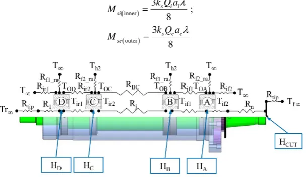
[image:3.595.163.467.518.694.2](4)
where ks is the friction coefficient, ae, ai are the major axes of the inner and outer contact ellipse area and λ is the contact area geometry factor [6]. The heat generation in the inner ring Hik and outer ring Hek con-tact zone for ball k, is found from the power loss equation, where power is rotational speed times moment.
roll roll
; .
ik fi si si
ek fo se se
H M M
H M M
ω ω
ω ω
= +
= + (5)
It is assumed that for grease lubrication all heat generation enters the combined ball/ring network. The overall bearing heat generation is the summation of the contact heat generation at the inner and outer rings [8]. The housing will experience the heat generated from the outer ring He, while the spindle shaft receives heat gener-ation from the inner ring Hi.
1 1
,
b b
N N
i ik e ek
k k
H H H H
= =
=
∑
=∑
(6)where Nb is the total number of balls in the bearing. The Hertzian contact theory is used in this study to com-pute the contact loads Qi, Qe between bearing balls and bearing rings. The Hertzian inner and outer contact loads for each ball are shown inFigure 2 and expressed by [12]-[14]:
3 2 3 2
;
ik i ik
ek o ok
Q K
Q K
δ δ
=
= (7)
where k is the ball index, δik, δok are the relative normal contact displacement between ball, inner and outer ring. Ki and Ko, the load deflection parameters can be obtained using the equations shown in Appendix A
[11] [14].
The bearing displacement vector
{ }
δ describes the three linear and two rotational motions, δ δ δ γ γx y z y zT. Due to the external forces applied to the bearings, displacements appear within the inner and outer rings and the distance between the curvature centers of the bearing rings change, as shown inFigure 3 [14]. The relative dis-placement between the inner ring and the outer ring can be expressed as:0
; o; i o; i o; i o
x y y z z z y y y z z
i i
x x y z
δ
δ
δ
δ
δ
δ
δ
δ δ
γ
γ
γ
γ
γ
γ
∆ = − ∆ = − ∆ = − ∆ = − ∆ = − (8)
where Bd is the distance between the curvature centers of the inner and outer rings before deformation of the bearing and can be represented as:
(
o i 1)
.d
B =BD= f + −f D (9)
; in ou i o r r f f D D
= = (10)
As shown inFigure 3, where k is the ball index. ∆ik and ∆ok can be expressed as:
(
)
(
)
;
2 0.5
2 0.5 .
ik in ik in ik
ok ou ok o ok
r D f D
r D f D
δ δ
δ δ
∆ = − + = − +
∆ = − + = − + (11)
The following relations are derived fromFigure 3:
(
)
(
)
(
)
(
)
sin ; 0.5 cos ; 0.5 sin ; 0.5 cos . 0.5 k ok o ok k ok o ok ik k ik i ik ik k ik i ik U r D DV r D D
U U r D D
V V r D D
θ δ θ δ θ δ θ δ = − + = − + − = − + − = − + (12)
Figure 2. Angular contact ball bearings. (a) Geometry and temperature terms; (b) Loads diagram [15]; (c) Forces acting on the bearing ball [14].
Figure 3. Displacement relationships between curvature centers of bearing rings under load [14].
cos sin cos sin 0;
sin cos sin cos 0
gk gk
ok ok ok ik ik ik ck
gk gk
ok ok ok ik ik ik
M M
Q Q F
D D
M M
Q Q
D D
θ θ θ θ
θ θ θ θ
− − + − =
+ − − =
(13)
where Fck and Mgk are the centrifugal force and gyroscopic moment, respectively [14]. The displacement equations for the bearing ball as shown inFigure 3 can be expressed as [14]:
(
) (
)
( ) ( )
2 2 2
2 2 2
; 0 0.
ik k ik k ik
k k ok
U U V V
U V
− + − − ∆ =
+ − ∆ = (14)
(a) (b)
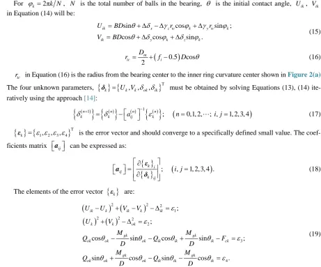
[image:5.595.198.428.340.542.2]For ϕ =k 2πk N, N is the total number of balls in the bearing, θ is the initial contact angle, Uik, Vik
in Equation (14) will be:
sin cos sin ;
cos cos sin .
ik x z ic k y ic k
ik y k z k
U BD r r
V BD
θ δ γ ϕ γ ϕ
θ δ ϕ δ ϕ
= + ∆ − ∆ + ∆
= + ∆ + ∆ (15)
(
0.5)
cos2
m
ic i
D
r = + f − D θ (16)
ic
r in Equation (16) is the radius from the bearing center to the inner ring curvature center shown inFigure 2(a).
The four unknown parameters,
{ } {
δk = U Vk, k,δ δ
ok, ik}
T must be obtained by solving Equations (13), (14)ite-ratively using the approach [14]:
( )
{ }
{ }
( ) ( ) 1{ }
( )(
)
1
; 0,1, 2, ; , 1, 2, 3, 4
n n n n
k k aij k n i j
δ + = δ − − ε = =
(17)
{ } {
}
T1, 2, 3, 4
k =
ε ε ε ε
ε is the error vector and should converge to a specifically defined small value. The
coef-ficients matrix aij can be expressed as:
{ }
{ }
k i ;(
, 1, 2, 3, 4 .)
ij
k ij
i j
= ∂
=
∂
ε a
δ (18)
The elements of the error vector
{ }
εk are:(
) (
)
( ) ( )
2 2 2
1
2 2 2
2
3 4
; ;
cos sin cos sin ;
sin cos sin cos .
ik k ik k ik
k k ok
gk gk
ok ok ok ik ik ik ck
gk gk
ok ok ok ik ik ik
U U V V
U V
M M
Q Q F
D D
M M
Q Q
D D
ε ε
θ θ θ θ ε
θ θ θ θ ε
− + − − ∆ =
+ − ∆ =
− − + − =
+ − − =
(19)
The bearing’s contact loads Qik, Qok in Equation (7) are obtained using the calculated values of
{ }
δk . The bearing heat generation can be computed by Equations (2)-(6) using the calculated variables values. Knowing the bearing heat generation quantity, we can move forward to the thermal model of spindle and housing.2.2. Spindle and Housing Thermal Model
The developed model is based on representing the spindle and the housing using axisymmetric thermal resis-tance elements. For the solution, the input parameters are: geometry, material parameters, air temperature, heat generation due to the bearings and initial temperature of the system. The thermal resistance is calculated for each housing and spindle element. Linear thermal resistance is defined according to the following equation [6]:
L R
KA
= (20)
where L is the element length, K is the material thermal conductivity and A is the cross-sectional area.
[image:6.595.77.539.87.470.2]2.2.1. Bearing Heat Transfer Model
Figure 4shows the bearing geometry and temperature nodes definition as well as the bearing heat transfer mod-el. The externally driven spindle is grease lubricated. With grease-packed lubrication, heat convection is less significant and conduction is more prominent. The radial heat transfer through the spindle, rolling element and housing is described similar to the thermal resistance network described by Jorgensen [6] and is shown in
Figure 4. Bearing heat resistances model.
(
)
(
)
(
)
(
)
1 2 2 2 1 1 ; ; ; ; 1 12π π 2π π π
ln ln
1 1 1
; ; .
1 1 2π
2 2 2 2 2 2π 2 Le b b b
Li Le b
b b Le b
l i i b l e e b
Le b
Li b o e i s
e i
Li b e i
Li b
R R
r r
R R R R
k r R R
k rW r k r W r
R R
n n
R R n r r n r r
R R R
R R k W k W
R R = = = = = + − − + = = = = + + (21)
The heat transfer equations use temperatures at the edge of the inner and outer rings as boundary conditions. As an alternative solution method, the outer ring temperature can be easily measured and applied to the solution, allowing the housing approximations to be ignored. Steady state outer ring temperatures can be used to provide a reference point for the thermal equations [6]. The matrix form of the heat transfer equations can be expressed as:
[ ]
Rb{ } { }
T = H (22)where
[ ]
Rb is the system heat resistance matrix;{ }
T is the vector of unknown temperatures, in this case three unknowns, and{ }
H are the heat generation inputs. As shown inFigure 4, Equation (22) can be written as:11 12 21 22 23
32 33
0
0.0 0
b b Le Le e O e
b b b b b
b b Li Li i i i
R R T H H T R
R R R T H
R R T H H T R
+ = = + (23)
The resistance matrix elements, Rbij as well as the expressions for the generated heat can be found in Ap-pendix B. Solving Equation (22) allows to predict the contact points’ temperatures TLe, TLi as well as the bearing ball temperature Tb. Although the heat transfer equations are approximations, sufficient accuracy is at-tainable for thermal expansion predictions [6].
2.2.2. Housing Heat Transfer Model
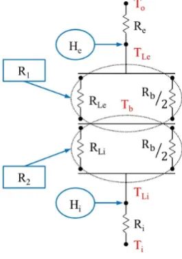
The housing heat transfer model based on quasi-two-dimensional analysis of heat flow is shown inFigure 1. The geometry parameters are shown inFigure 5. The four unknown nodal points’ temperatures, ToA, ToB, ToC,
oD
T , shown inFigure 1, were calculated by applying axial and radial conduction and convection resistance ele-ments. The radial and axial resistances for an element can be expressed as:
rad air ln 1 ; 2π 2π h o h h r r R
k L h L r
= + (24)
(
2 2)
(
2 2)
1
π π
ax
h h o air h o
L R
k r r h r r
= +
− − (25)
[image:7.595.243.384.590.670.2]Figure 5. Spindle and housing 2D configuration.
ends in the element. In order to simplify the heat transfer equilibrium equation the axial and radial element re-sistance are combined as shown in the following equation:
rad total
rad
ax ax
R R R
R R
× =
+ (26)
total
R is the element total resistance. The housing heat transfer equations in matrix can be expressed as:
[ ]
Rh{ } { }
T = H (27)where RA and RD are the total resistance of the front and rear housing elements. RBC_rad is the resistance of the connection element between points B and C. The resistance matrix elements Rhij as well as the expressions for generated heat and the resistances RA, RD and RBC_ rad can be found in Appendix C. By solving the set of Equation (27), the temperature values at the four most heated points along the housing outside surface are ob-tained.
2 11 12
_rad 21 22 23
32 33 34 2
_rad 43 44
0 0
0
0
0 0
OA A h
h h OA
OB BC
h h h OB
h h h OC h
OC BC
h h OD
OD D
T H
R T
R R T
H R
R R R T
R R R T T
H R
R R T
T H
R ∞
∞
+
+
=
+
+
(28)
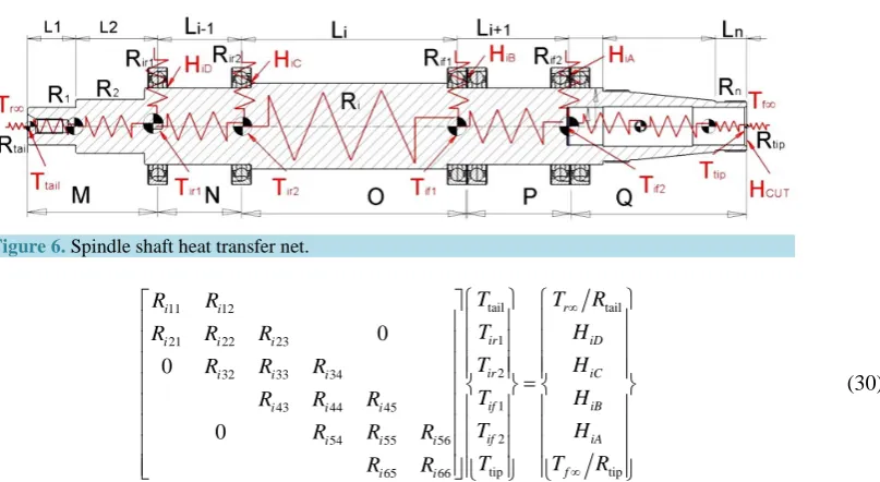
2.2.3. Spindle Shaft Heat Transfer Model
As shown inFigure 6, the spindle shaft is represented by a nine resistance element model. By applying the same matrix notation as above, the matrix notation of the heat generation balance is obtained:
[ ]
Ri{ } { }
T = H (29)Figure 6. Spindle shaft heat transfer net.
tail tail 11 12
1 21 22 23
2 32 33 34
1 43 44 45
2 54 55 56
tip tip
65 66
0
0 0
r
i i
ir iD
i i i
ir iC
i i i
if iB
i i i
if iA
i i i
f
i i
T T R
R R
T H
R R R
T H
R R R
T H
R R R
T H
R R R
T T R
R R
∞
∞
=
(30)
All matrix and vector elements presented in Equation (30) are expressed in Appendix D. By solving the set of Equation (30), the temperature values in six points of interest along the spindle shaft centre are obtained.
3. Experimental Setup for Spindle System Analysis
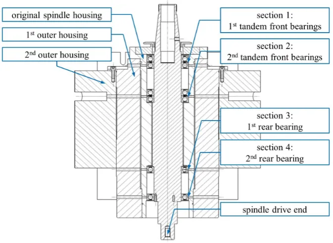
The configuration of the test rig used for experimental investigations of an externally driven spindle is shown in
Figure 7andFigure 8. An air-cooled asynchronous motor is connected via an elastomer coupling to the spindle. In addition to the original spindle housing two adjacent outer housings were used to mount the spindle on to the test rig.
The motor, friction in the bearings and the cutting process are the main causes of heat generated by the spindle system during machining operation. The motor is cooled using air flow in the direction from the drive end of the motor to the non-drive end. By assuming that most of the cutting heat is taken out by the coolant and that the heat generated by the motor in the configuration shown inFigure 7 andFigure 8 is kept away from the machine tool spindle, it follows that the heat generated by the bearings is the dominant heat source causing the thermal distor-tion of the spindle shaft. The motor’s maximum continuous duty speed is 7000 rpm, with a rated power output of 12 kW. During machining operations such as external cylindrical rough grinding high cutting capacity is required, while during fine grinding a high standard of form and surface quality should be maintained. In order to achieve both mentioned requirements a high degree of rigidity and running accuracy as well as good damping and speed suitability are the main criteria for the spindle bearing arrangement. These requirements are met by the precision bearings assembled in the test spindle. Sealed universal spindle bearings with small steel balls (HSS) are used:
• at the tool end: 1 spindle bearing set, in double O arrangement (Tandem), as fixed bearings
• at the drive end: 1 spindle bearing set, in O arrangement, as floating bearings
The employed contact angle of 15˚ is suitable for high radial rigidity. The universal design bearings are lightly preloaded. The sealed spindle bearings require no maintenance and are lubricated for life with roller bearing grease [5].
Figure 7. Test rig configuration for the externally driven grinding spindle.
Figure 8. Experimental setup of the sensors and the data acquisition arrangement.
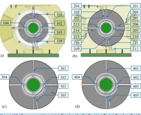
Figure 10. Sensor positions: (a) Section 1; (b) Section 2; (c) Section 3; (d) Section 4.
Figure 10 and the wiring is shown inFigure 8. As mentioned before, the only heat source within the spindle system, during the externally driven spindle operation in the configuration described above is the bearing friction. The heat generation of internal components as a function of spindle speed is only investigated using the test rig described. The research phase is applied in order to gain fundamental knowledge about the heat generation in the spindle system with less complexity. The next step of the investigations will include load-dependent heat genera-tion and heat flux as well as the motorized spindle system’s thermal behavior.
4. Spindle System Thermal Behavior—Experimental Study
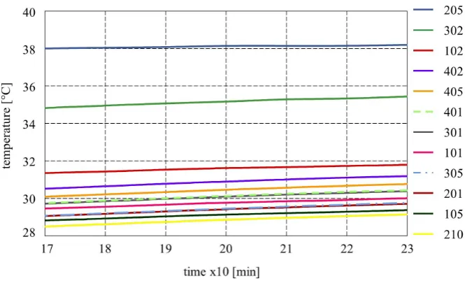
The thermo-elastic behavior of a machine tool is strongly nonlinear and has to be modelled for several operating points. Hence, the speed spectrum has to be divided into several sections, each having its own operating point [2]. Sensitivity analysis under variety of operating modes has been designed and carried out. The spindle speed spec-trum up to 7000 rpm is divided into seven operating points starting at 1000 rpm with steps of 1000 rpm. The du-ration of a single step was chosen to be 4 h. The sensor area with the highest temperature in each measurement section was the one located on the bearing outer ring.Figure 11 illustrates the highest measured temperature ob-tained at spindle speeds from 1000 to 7000 rpm. The sensors mounted in Section 2 present the highest tempera-ture over all spindle speeds. Figure 12 illustrates the steady state temperatures measured in the sections men-tioned above according to 3 sensor measurements in each section at 7000 rpm spindle speed. Sensor no. 205 mounted in section 2 at the position directly adjacent to the bearing outer ring. In this position the highest temper-ature (38.2˚C) was achieved. The second highest temperature, 35.4˚C, was measured by sensor no. 302 and 31.8˚C was measured by sensor no. 102. All 3 sensors mentioned above were mounted in touch with the bearing’s outer ring in each section. As shown inFigure 10, 16 sensors are mounted in Section 2. The graph inFigure 13
represents the temperature measured in 5 of the 16 different sensor positions in Section 2. All points across the section from the deepest measuring point, the outer bearing ring, through all 3 housing elements, to the outermost measuring point (sensor no. 204), were heated. Even the outmost point on the outer housing in the 2nd section was affected by the heat generated due to the bearing friction.
By changing the spindle speed over the speed spectrum, from 1000 rpm to 7000 rpm, it is clear fromFigure 14
that the highest rate of change in the maximum temperature occurs when the rotational speed is increased from 5000 to 7000 rpm.Figure 15 illustrates the influence of spindle speed on the measured temperature in Section 2, sensors no. 201 to 205. As already mentioned, the thermo-elastic behavior of the main spindle system in a ma-chine tool is strongly nonlinear and has to be investigated and modelled in several simplifying steps. First, the thermal behavior of an externally driven spindle was investigated in order to verify and apply a simple simula-tion model, based only on the heat generated by the fricsimula-tion in the bearings. The heat flux from the bearings into
(a) (b)
Figure 11. Measured temperature in the most heated sensors among all sections over ch- anging spindle speeds.
Figure 12. Measured temperature at steady state in 4 Sections; 3 sensors each section.
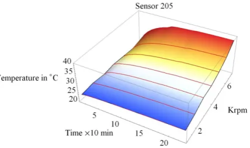
[image:12.595.147.480.281.482.2] [image:12.595.146.479.507.704.2]Figure 14. Temperature measured by sensor no. 205, as a function of time and spindle speed.
Figure 15. Measured temperature in Section 2 while changing the spindle speed from 3.000 to 7.000 rpm.
several outer housings is investigated as well. By verifying the heat transfer from the inner bearings element to the outer housings, one is able to understand the heat flux mechanism and the influence of the heat generated in the bearings on the spindle-adjacent machine elements.
5. Numerical Simulations
Based on the model described in Section 2 and Appendices A to D, a simulation program was developed. The numerical computations as well as the graphical presentations and investigations were carried out using the Ma-thematica® software [16]. Using the algorithm and software developed, numerical studies of the heat transfer mechanism and temperature variations along the external driven spindle system were made. Some simplifica-tions were made in the simulation programs above. No motor and no external cutting load exists in this stage of the study, in order to enable the use of this model as a base line for further simulations including the cutting process effects and motorized spindle simulations.
5.1. Validation of the Simulation Model
[image:13.595.163.463.263.443.2]stu-dies described in Section 4. The numerical simulations investigate the effect of operating conditions such as ro-tational speed (rpm), axial preload, lubricant viscosity, as well as geometrical parameters of the spindle system structural components. Comparison between measured temperatures at the housing outer surface, sensors 101, 201, 301 and 401, and simulated temperature along the axis of the spindle system in the bearings’ positions is shown inFigure 16 andFigure 17 for different ranges of spindle rotational speeds.
From Figure 16andFigure 17 it follows that there is a good fit between the simulation results and the expe-rimental results obtained. It can be seen that the differences are in the range of 1˚C to 2˚C over the full range of spindle speeds. It should be mentioned that the main goal of the simulation model is to be fast and efficient and should give first approximation only during an early stage of spindle design. It should not be accurate as a FEM or other simulation software programs, which are much more complex and time consuming.
5.2. Simulations under Speed Variations
Internal heat generation and heat flow is strongly speed-dependent.Figure 18 shows the temperature developed in the spindle housing outer surface, ToA, ToB, ToC, ToD, at the sections shown inFigure 10. The results can be achieved only by simulation because the spindle and bearings speed limit is 7000 rpm.
The temperature profiles inFigure 19 identify the temperatures Tle in the ball bearings’ point of contact with the outer and inner rings. These contact points show the highest temperature within the spindle system.
Figure 16. Comparison between measured temperatures and simulated temperature as a function of spindle speeds between 2.000 and 4.000 rpm.
[image:14.595.147.480.306.481.2] [image:14.595.147.481.516.694.2]the bearing balls and the bearing outer ring. According to the developed model and as mentioned in the lite-rature [6], it is assumed that part of the heat generated in the contact flows into the bearing ring and another part flows into the bearing ball.Figure 21 shows the temperature profile along points of interest along the spindle shaft axis, as shown inFigure 6, for various spindle rotational speeds.
Figure 18. Simulated temperature at changed spindle speed up to 30.000 rpm.
Figure 19. Simulated temperature Tle at the contact point between the
[image:15.595.178.447.354.522.2]bearing ball and the bearing outer ring.
[image:15.595.212.415.561.696.2]Figure 21. Simulated temperature at 6 points along the spindle shaft axis.
Ttail, Tir1, Tir2, Tif1, Tif2, Ttip over spindle speeds spectrum from 2.000 to
7.000 rpm.
6. Conclusions
The theoretical and experimental investigations of the heat transfer mechanism in the externally driven grinding spindle have enabled the following conclusions.
1) The use of the bearing heat generation terms in each model, bearing model, spindle model and housing model enabled investigation of the thermal behavior of the entire spindle system under the effect of the main source of heat generation: the bearings’ friction.
2) Experimental investigation of the heat transfer in the spindle system and the machine elements adjacent to the spindle allows obtaining the data needed for better understanding the heat generation and flux due to the bearing friction.
3) The simplifying assumptions of the method presented in this study are mainly the one-dimensional heat flow approximations, simplified housing geometry, external drive motor, excluding the cutting process heat and excluding cutting process loads. These spindle-housing approximations are acceptable since the most important temperature predictions are those within the bearings.
4) Using the models presented, the temperature field can be numerically found for most spindle-housing configurations in a fast and efficient manner. The simulated and validated temperature fields can be used for numerical simulations of spindles thermal expansion and machine elements adjacent to the spindle, as well as for machine tool precision prediction during the development process.
Acknowledgements
The Authors want to thank the DFG (German Research Foundation) for financial support. The represented find-ings result from the subproject B03 “Investigation of Components and Assembly Groups” of the special research field SFB/Transregio 96 “Thermo-energetic design of machine tools”.
References
[1] Brecher, C. andWissmann, A. (2011) Compensation of Thermo-Dependent Machine Tool Deformations Due to Spin-dle Load: Investigation of the Optimal Transfer Function in Consideration of Rough Machining. Production Engineer-ing, 5, 565-574. http://dx.doi.org/10.1007/s11740-011-0311-4
[2] Bryan, J. (1990) International Status of Thermal Error Research. CIRP Annals—Manufacturing Technology, 39, 645- 656. http://dx.doi.org/10.1016/S0007-8506(07)63001-7
[3] Mayr, J., Jedrzejewski, J., Uhlmann, E., Donmez, M.A., Knapp, W., Härtig, F., et al. (2012) Thermal Issues in Ma-chine Tools. CIRP Annals—Manufacturing Technology, 61, 771-791.
http://dx.doi.org/10.1016/j.cirp.2012.05.008
Dynamic Thermo-Mechanical Spindle Model. International Journal of Machine Tools and Manufacture, 44, 347-364. http://dx.doi.org/10.1016/j.ijmachtools.2003.10.011
[6] Jorgensen, B. (1996) Robust Modeling of High-Speed Spindle Bearing Dynamics under Operating Conditions. Ph.D. Thesis, Purdue University,West Lafayette.
[7] Palmgren, A. (1959) Ball and Roller Bearing Engineering. 4th Edition, S.H. Burbank, Philadelphia.
[8] Bossmans, B. and Tu, J. (1999) A Thermal Model for High Speed Motorized Spindles. International Journal of Ma-chine Tools and Manufacture, 39, 1345-1366. http://dx.doi.org/10.1016/S0890-6955(99)00005-X
[9] Li, H. and Shin, Y.C. (2004) Integrated Dynamic Thermo-Mechanical Modeling of High Speed Spindles. Part 1: Mod-el DevMod-elopment. Journal of Manufacturing Science and Engineering, 126, 148-158.
http://dx.doi.org/10.1115/1.1644545
[10] Kim, J.D., Zverv, I. and Lee, K.B. (2003) Thermal Model of High-Speed Spindle Units. KSME International Journal, 17, 668-678.
[11] Harris, T.A. (1991) Rolling Bearing Analysis. 3rd Edition, John Wiley & Sons, Hoboken.
[12] Zhao, H.T., Yang, J.G. and Shen, J.H. (2007) Simulation of Thermal Behavior of a CNC Machine Tool Spindle. Inter-national Journal of Machine Tools and Manufacture, 47, 1003-1010.
[13] Harris, T.A. and Kotzalas, M.N. (2005) Advanced Concepts of Bearing Technology, Rolling Bearing Analysis. 5th Edition, Taylor & Francis Corporations, London.
[14] Cao, Y. (2006) Modeling of High-Speed Machine-Tool Spindle System. Ph.D. Thesis, British Columbia University, British Columbia.
[15] Altintas, Y. and Cao, Y. (2005) Virtual Design and Optimization of Machine Tool Spindles. CIRP Annals—Manu-
facturing Technology, 54, 379-382.
Appendix A
(
) (
)
(
)
0.636 2 2 2 π ; 3 1.03391.5277 0.6023ln ;
1.0003 0.5968 ;
2 ; 1 1 . ; xy y x x y x y a b x y xy x y R E K R R R R R R E Ea Eb R R R R R κ κ µ µ ′ = = = + = + ′ = − − + = + E F F F
E (A.1)
where µa, µb are Poisson’s ratio of the bearing ball and the rings, respectively. For the inner and outer ring contacts, Rx and Ry are:
(
)
(
)
1
; ;
2 2 1
1 ; ;
2 1 2
cos cos ; . ik ou xik xok ou ok in yik yok in ik ok ik ok m m
D D f
R R f D D f R R f D D D D γ γ θ θ γ γ − ⋅ = = − + ⋅ = = − = = (A.2)
Appendix B
1 1 2 2
; ;
Le o Le b b Le b Li Li b Li i
e b i
e R R i
T T T T T T T T T T T T
H H H
R R R R
− − − − − −
= + = + = + (B.1)
11 12 21 22 23
1
32 33
1 1 1 2 2
2 2
1 1 1 1 1 1 1
; ; ; ; ;
1 1 1
; .
b b b b b
e
b b
i
R R R
R R R R R
R R
R R
R R
R R R
= + = − = − = + = −
= − = +
(B.2)
Appendix C
total total total rad
2
; ;
ax
oD oD oC oC oD oC oB oC h
oD oC
D C C BC BC
T T T T T T T T T T
H H
R R R R R
∞
− − − − −
= + = + + (C.1)
2
_ _rad _total _total _total
; ;
oB oC oB h oB oA oA oA oB
oB oA
BC ax BC B A B
T T T T T T T T T T
H H
R R R R R
∞
− − − − −
11 12
21 22 23
_ _ _
32 33 34
_ _ _
43 44
; ;
1 1 1 1 1
; ; ;
1 1 1 1 1
; ; ;
1 1 1
; .
h h
A B B
h h h
B B BC ax BC rad BC ax
h h h
BC ax C BC ax BC rad C
h h
C C D
R R
R R R
R R R
R R R R R
R R R
R R R R R
R R
R R R
= + = − = − = + + = − = − = + + = − = − = + (C.3)
(
)
(
)
(
)
(
)
1_ 2 2 2 2
_rad
1 1
2
_ 2 2 2 2
_rad 2 2 2 1 ; π π ln 1 ; π π 1 ; π π ln 1 2 . π π 2 2 f A ax
h Ah Ao air Ah Ao
Ah Ao A
h f air f Ah
r D ax
h Dh Do air Dh Do
Dh Do D
h r air r Dh
L R
k r r h r r
r r R
k L h L r
L R
k r r h r r
r r R
k L h L r
= + − − = + = + − − = + (C.4)
Housing free convection [6]:
(
)
(
)
(
)
1 3 2_ 2 2
_rad
2 2
1
_ 2 2
_rad 1 1 _rad _ 17.63 ; 0; π ln 1 ; π π 0; π ln 1 ; π π ln 1 ; 2 2 2 π 2
2 2π
air
f B ax
h Bh Bo
Bh
Bo B
h f air f Bh
r C ax
h Ch Co
Ch
Co C
h r air r Ch
BCh
BCo BC
h air BCh
BC ax
h T T
L R
k r r
r r R
k L h L r
L R
k r r
r r R
k L h L r
r r R
k L h L r
R ∞ = − = + − = + = + − = + = +
(
2 2)
0.π
h BCh BCo
L
k r r
= +
− (C.5)
_ _rad _ _rad
_total _total
_ _rad _ _rad
_ _rad _ _rad
_total _total
_ _rad _ _rad
; ;
; .
A ax A B ax B
A B
A ax A B ax B
C ax C D ax D
C D
C ax C D ax D
R R R R
R R
R R R R
R R R R
R R
R R R R
Appendix D
2 1
tail tail 1 1 tail 1 2 2 1
1 2 1 2 2
t
1 2 2
ail
0 ; ; ;
; ; 0 .
ir if
r ir ir ir ir ir ir
iD iC
M M N N O
if ir if if if if if tip tip if tip f
iB iA
O P P Q Q tip
T T
T T T T T T T T T T
H H
R R R R R
T T T T T T T T T T T T
H H
R R R R R R
R ∞ ∞ − − − − − − = + = + = + − − − − − − = + = + = + (D.1) 1 1
1 1 2 1
1 2 1
1 2 3 1 2
1 1 1 1
2 1 4 2 1
2 1 2 1
1 2 5 1 2
1 1 2 1
1 1
2 2
1 1 1 1
;
2 2 2 2
1 1 1 1
2 2 2 2
1 1 1 1
;
2 2 2
;
; 2
ir
M j ir ir
j
ir
N j ir ir ir ir
j ir if
O j ir if ir if
j ir if
p j if if if if
j if
n
Q j if
R R R R R R
R R R R R R R
R R R R R R R
R R R R R R R
R − = − = + − = + − = + = + = + = + + = + + = + + = + + = + + = + + = + + =
∑
∑
∑
∑
∑
2 6 7 21
2 2 .
1
j if if
R + R =R +R + R
(D.2)
11 12
21 22 23
32 33 34
43 44 45
54 55 56
65
1 1 1
; ;
1 1 1 1
; ; ;
1 1 1 1
; ; ;
1 1 1 1
; ; ;
1 1 1 1
; ; ;
i i
tail M M
i i i
M M N N
i i i
N N O O
i i i
O O P P
i i i
P P Q Q
i
R R
R R R
R R R
R R R R
R R R
R R R R
R R R
R R R R
R R R
R R R R
R = + = − = − = + = − = − = + = − = − = + = − = − = + = −
= − 1 ; i66 1 1 .
Q Q tip
R
R = R +R
![Figure 2. Angular contact ball bearings. (a) Geometry and temperature terms; (b) Loads diagram [15]; (c) Forces acting on the bearing ball [14]](https://thumb-us.123doks.com/thumbv2/123dok_us/8167518.807731/5.595.198.428.340.542/figure-angular-contact-bearings-geometry-temperature-diagram-bearing.webp)