Energy Efficiency Behavior in Heterogeneous Networks under Various Operating Situations of Cognitive Small Cells

http://dx.doi.org/10.4236/wet.2015.61002

Energy Efficiency Behavior in

Heterogeneous Networks under Various

Operating Situations of Cognitive Small Cells

Amr A. Fahmy

1

, Asmaa M. Saafan

2

, Hesham M. El-Badawy

2

, Salwa El-Ramly

1

1_{Faculty of Engineering, Ain-Shams University, Cairo, Egypt} 2_{National Telecommunication Institute (NTI), Cairo, Egypt}

Email: [email protected], [email protected], [email protected], [email protected]

Received 30 December 2014; accepted 16 January 2015; published 19 January 2015

Copyright © 2015 by authors and Scientific Research Publishing Inc.

This work is licensed under the Creative Commons Attribution International License (CC BY). http://creativecommons.org/licenses/by/4.0/

Abstract

Recently, several approaches were followed for the enhancement and better resource utilization in mobile networks; this is to achieve energy efficient consumption for production and delivery of an information bit. Using Cognitive Femto cells (as a member of the small base stations’ family) proves that, it is an efficient solution for achieving this goal [1]. The use of Energy Efficiency term

( )

η has become one of the major indices for measuring the performance of these systems.

η

is the measure of the overall system Capacity

( )

C in bps/Hz versus the Consumed Energy

( )

E in

Keywords

Energy Efficiency, Capacity, Energy, Cognitive Radio, Wireless Communications, Green Radio

1. Introduction

Recently, huge interest has evolved for finding means to conserve the natural resources especially in communica-tions. Two facts are realized by communication systems’ engineers and researchers: the rapid consumption of natural resources and the increase in global warming with the dependency growth of civilizations on energy for using wireless communication systems, together, the scarcity of spectrum resources of these wireless communica-tion systems. “Green Communicacommunica-tion” is currently one of the hottest topics in the field of wireless communicacommunica-tion researches due to its contributions in saving the environment [3] [4]. “Energy Efficiency

( )

η ” is a major index suggested by EARTH’s Energy Efficiency Evaluation Framework (E3F) [5]- [8]; it is pursuing methods for saving energy consumed in accomplishing communications, which reduces pollution and preserves natural resources. Forthcoming mobile Generations will face many tradeoffs between the

η

considerations versus system perfor-mance parameters especially throughput. Cognitive Radio (CR) is one of the most elected techniques to be recog-nized as a candidate technology to implement Heterogeneous Networks (HetNet) Communications with better

η

. This paper illustrates different aspects that affect the

η

behavior. These parameters include Cognitive Base Sta-tions (CBS) radii (which will directly affect the CBS coverage area) and the distance between these CBSs from Macro Base Stations (MBS). A combination of analytical and simulation methods has been adopted to accom-plish the aimed target of the current work. Simulation scenarios are performed to illustrate the contribution of these parameters in the whole system Energy Efficiency.

The paper is organized as follows: Section 2 will introduce the CR based HetNet and its relation to the

η

index for CR networks. Section 3 proposes a system model and assumptions that will be adopted to evaluate the

η

index analytically. Whereas, Section 4 presents the performance evaluation and model validation, in which, main design milestones for the different simulation scenarios are illustrated. Section 5 previews the obtained re-sults and give detailed analysis about these rere-sults. Finally, Section 6 concludes the paper and gives the future directions for such area of interest.

2. Literature Review

3. System Model and Assumptions

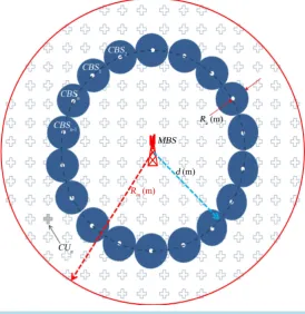
The system model elements are shown in Figure 1, a Macro-Base Station (MBS) is situated at the origin of the system, this MBS is assumed to cover a circular area, MBS operation parameters are shown later in Section 4. The downlink channel is assumed to follow the space loss model such that [15]:

out

r

P =P d−α (1)

where, P_r, is the received power at the receiver side, Pout, is the antenna output radiated power at the

transmit-ter side, α, is the free space path loss exponent, d is the distance between the transmitter and receiver anten-nas.

User Equipments (UE) joining this system model are either Macro Users (MU), where they are served by the MBS, or, Cognitive Users (CU) where they are served by the nearest CBS. They are all deployed uniformly in the MBS coverage area (locations are shown as “+” sign). N_UE is the total number of UEs, and is comprised of

MU

[image:3.595.161.436.430.713.2]

N and N_CU users and are shared between MBS and CBSs respectively. Those UEs are assumed to be sta-tionary (no mobility models used). Operational parameters of those UEs (MU or CU) are shown later in Section 4. CBSs are deployed uniformly at equal distances d from MBS situated at the origin of the system, this equal distance is meant to simulate the average (mean) distance for those CBSs uniformly distributed over MBS cov-erage area, in addition, their covcov-erage areas are not supposed to overlap. The number of CBSs

( )

n_C depends on how far from MBS they are situated, and, their cell coverage radii R_c. The larger R_c and the shorter d, the smaller number of CBS deployed and vice-versa. The non-overlapped CBS will give the nearest resem-blance to those CBSs deployed over a Voroni-tessellation scheme [16] [17]. A single Primary User (PU) at the MBS cell edge is considered, this PU will perform the interference as an adjacent cell interferer to MBSs’ fre-quency. This PU no traffic activity probability P_idle equals 0.4. Interference among system elements is assumed too; there are several interference types that are illustrated and considered in the next section. Moreover, R_c, d, n_C, will be varied through the simulation processes to find those major effects over the system

η

compo-nents. This assumed model was previously-more or less-introduced and used by multiple works [12] [18]. For model realization (without loss of generality) no resource management system will be applied. In addition, no legacy femto cells exist within the same MBS coverage area. There are F_M frequencies provided by MBS for

usage by UEs, those UEs go through two states of operation, active and idle with active probability

λ

. For MBS, and in order to apply

η

concepts, we need to reduce its radiated power to the needed level, i.e., the out-put power depends on the traffic load (active macro-users active

m

n ), such that:

(

)

out active max

tx

M M m m

P =P n n (2)

where, tx M

P is the radiated power depending on the linked active UEs, out

M

P is the maximum radiated power,

max

m

n is the maximum allowable served users by MBS. In this work max

m

n is assumed to be 300 users. For CBSs, the operational parameters used are given in Section 4. In [14], Channel switching cost is a linear func-tion of the difference between the current and the “be switched to” frequencies. The average number of channel switching δ_F is involved in calculating the cost of RF antenna tuning (channel switching cost). Here in this work (Section 3.3) it is assumed to be equal to 5. All the parameters used in this work are considered based on the available knowledge of the practical deployment in the urban areas. Also, these parameters are in consis-tence with [13]. For channel modeling parameters, the space path loss exponent α for communication chan-nels between macro-affiliated system components and cognitive-affiliated system components (i.e. cross layer communications and interference) are assumed to be equal to 2.8, while in mutual layer (co-layer) communica-tion and interference among cognitive-affiliated system components α is assumed to be equal to 2. This path-loss exponent difference is due to the different nature of working environment of both cases (MBS-UE, or, CBS-UE).

3.1. Capacity

Theoretically, capacity C=R W, where R is the bit rate and

W

is the used bandwidth. Basically,

C

is calculated using Shannon’s theorem which states that [19] [20]:

(

)

2

log 1 SNR

R

W = + (3)

In this work, theoretical capacity is used to obtain the maximum capacity available by the system, further modifications may be applied to enforce conditions of the actual bit rate. R, is influenced by the received sig-nal to noise ratio, the noise is also influenced by the received interference from other system components oper-ating within the same frequency band.

3.2. Noise and Interference

In order to calculate the system capacity

C

, the different types of interference should be considered. Assuming that the system only consists of MBSs, CBSs, and a single PU located at the MBS cell-coverage edge, interfe-rence is limited to three types of interfeinterfe-rence, co-layer, cross-layer, and cognitive-layer [13]. The co-Layer In-terference occurs when a CBS transmitted signal extends to an adjacent CBS cell causing inIn-terference to the neighbor CU operating at the same frequency. The cross-Layer Interference happens in the downlink between macro layer and cognitive layer, that is, when a MBS generates interference to the user receiving at the same frequency in the other layer (i.e. MBS to the CUs and CBS to the MUs). Finally, cognitive Layer Interference where CBS may receive severe interference from the external primary networks at small cell CR frequencies. This interference effect is significantly high in case of misdetection compared to the opportunistic use of the spectrum after successful discovery of the idle bands. In this work, interference is calculated as received signals’ strength from source BS to other BSs’ UEs. Signals received from other BS are subjected to the space loss mod-el mentioned before , moreover noise spectral density is calculated in its primitive form as:

0 , J/K

N = ⋅k T (4)

where, k is Boltzmann constant, T is the absolute temperature in K, and assuming the involved band width to be 10 MHz (in conformance with LTE standards [15] [21]). Signal to interference ratio is calculated by di-viding the received signals’ strength dis

Rx

P at BS/user dis operating at the same frequency by the interference plus noise, such that [15]:

dis src src,dis

Rx Tx

P =P ⋅G (5)

where, src stands for “source” and dis stands for “destination”, and src

Tx

transmitter src, Gsrc,dis is the channel fading gain between a source transmitter src and distant receiver dis due to a space loss model mentioned in (1). Following the analytical model in [13], the interference from multiple sources to a certain destination I_dis is the summation of all the received signals at the distant receiver (and within the same operational bandwidth) multiplied by the activity probability such that:

(src,dissrc,dis ) src,dis src,dis

dis 1 src

N n n

Tx n

I =

∑

₌ λ P G (6)

where, N_src,dis is the number of all active interference sources src causing interference to a single destination dis. Let F_src bethe total number of frequencies provided by src type BS, and λ_src be the probability of CU be-ing in active state, thus, the number of interferers as λ_src

(

N_src F_src

)

where N_src is the number of similar type nodes excluding the node itself. CBSs conduct a sensing procedure to allocate usable holes in the spectrum, the sensing period is performed once in each T_s time slots. The a detection probability p_d during this period is

( )

d s

p T . So, by suggesting that capital letters

C

, M denote CBSs and MBS, and small letters c, m,

p

denote CU, MU and PU respectively, and in consistence with [13]:

, , 0

m C m C m

I =n I +N , (7)

( )

(

)

, , , , , 1 , 0

c C c C c M c M c p c d s p c

I =n I +n I +n −p T I +N , (8)

where, I_m, Ic are the total interference at all users of macro and Cognitive stations respectively (either MU or CU). Assuming a probability of detection and false alarm for MBS frequencies within time slots T_s are [13]:

( )

0.9

(

1

)

d s s

p T = T − (9)

( )

0.1

(

1

)

fa s s

p T = T − (10)

Which are in consistence with [13]. Let F_M , F_C be the number of frequencies provided by MBS, CBS re-spectively, and n_m, n_c as the number of MUs, CUs respectively, it is now possible to get the obtained capac-ity of the various system components MU, CU, where:

2 log 1 rx m M m m m P F C n I   =  + 

  (11)

2

1

log 1

rx

s C c

c

s c c

T F P

C

T n I

 

−

= ⋅  + 

 . (12)

where, rx m P , rx

c

P are the received power at MU, CU from their affiliate MBS, CBS (respectively). Thus, the overall capacity of the system model components is:

m c

C=C +C (13)

3.3. Energy Consumption Estimation

[image:6.595.142.457.81.281.2]

Figure 2. Input power consumed by MBS system components Vs output RF power per-centage, considering: mains power supply (MS), cooling system (CO), DC-to-DC

con-verters (DC), baseband processor (BB), RF transceiver (RF), power amplifier (PA) [12].

(mains supply) for connection to the electrical power grid.

For BS Variable Load, (i.e. the power consumption of PA depends on the traffic load), it was found that BS power consumption model is shown in [12], or, an acceptable approximation for the power consumed by MBS is mathematically taken as a straight-line equation by:

(

)

in 0 out 0 out max

TRX ,

M M p M M M M

P =N ⋅ P + ∆ P P ≤P ≤P (14)

where, in

M

P denotes the overall power consumed by MBS, max

M

P is the maximum RF output power at maxi-mum load, 0

M

P is the power consumption calculated at the minimum possible output power (assumed to be 1% of max

M

P ), and ∆_p is the slope of the load dependent power consumption, N_TRX is the number of TRX chains. For MUs, power consumption depends on the traffic activity condition.

Assuming i m

P is the power consumption during idle state, λ_m is the active downlink probability, and

p

is the probability success to have an available (operative) frequency from MBS where p=F_M n_m (for,

M m

F ≤n ). So, CU equipment energy consumption E_m is:

(

1

)

rx i

m m m m m

E =

λ

pP + −

λ

p P (15)

3.3.1. Energy Consumption of CBSs

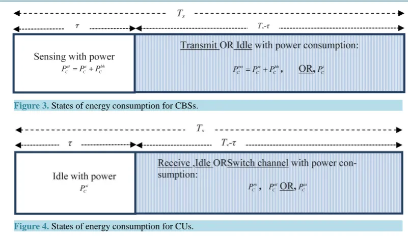
Figure 3 shows the different states of power consumption by a CBS. In an observation of a number of multiple normalized time slots T_s. A CBS functions in one of three modes, in the first mode, which is performed in a number of time slots τ, a CBS consumes power st

C

P to perform sensing peration for frequency holes with the maximum detection probability. In the second mode, which is performed during the remaining part of the avail-able time slots (i.e. T_s−τ), a CBS transmits power txt tx bh

C C C

P =P +P to a CU, where tx C

P is the consumed power for performing transmission to CUs, and bh

C

P is the consumed power to handle the backhaul require-ments. In the third mode, which is alternatively performed with the second mode and during the other part of

s

T −τ slots, a CBS consumes power i C

P during a state of idle. Let λ_c be the probability of a CBS being in the transmit state, so, the average energy consumed during T_s is:

(

)

(

txt

)

(

)

1

st i

C c C c C s

C

s

P P P T

E

T

τ+ λ + −λ −τ

= . (16)

3.3.2. Energy Consumption of CUs

[image:7.595.93.494.77.309.2]

Figure 3. States of energy consumption for CBSs.

Figure 4. States of energy consumption for CUs.

multiple normalized time slots T_s, a CU functions in one of three modes. The first mode occurs in a number of time slots τ, in which CBS performs sensing. CU consumes power to perform idle state si

c

P during a “CBS sensing period”. In the rest of the time slots T_s (i.e. T_s−τ), CU performs reception operation (traffic state) by consuming power rx

c

P . Allocated frequencies by CBS change with an average number of channel switching

F

δ , it takes cs c

P power to perform this channel switching. In the third mode which occurs during the same in-terval of time

(

T_s−τ

)

, CU consumes power ni

c

P during other “normal” states of idle when not in reception mode.

Let λ_c be the probability of a CU being in the traffic state, so, the average energy consumed during T_s is:

(

)

(

)

(

1

)

(

)

si rx cs ni

c c c F c c c s

c

s

P P P P T

E

T

τ

+

λ

+

δ

+ −

λ

−

τ

= (17)

The total energy consumption by the system model is:

M m m C C c c

E=E +n E +n E +n E , (18)

where, in

M M s

E =P T , n_m is the number of MUs, n_C is the number of CBSs, n_c is the number of CUs.

3.4. Energy Efficiency Estimation

Using Equations (13) and (18), energy efficiency

η

is calculated as:

C E

η = (19)

And since

C

is in bits/second/Hz, and E is in Joules, so,

η

is in bps/Hz/J.

4. Performance Evaluation and Model Validation

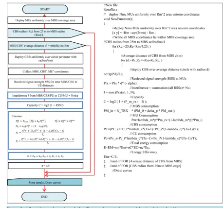
4.1. Proposed Algorithm and Parameters

[image:8.595.76.535.81.509.2]

Figure 5. A flow chart and pseudo code that illustrate the main features of the simulation algorithm.

4.2. Procedures

The assumed parameters are initialized with values shown in Table 1 and Table 2. Table 1 shows the MBS, UE, CBS assumed values of operating parameters. The average distance between CBSs and MBS d is varied at equal steps between 25 m and R_m (MBS cell radius). The smaller the average distance d the smaller the number of deployable CBSs because their coverage areas should not intercept. In addition, increasing R_c will lead to decreasing the number of CBSs deployed over the same d. To calculate the power consumed by MBS at variable load in

M

P , Equation (14) is used by substituting values from Table 2 which shows the assumed pa-rameters to approximate the power consumption behavior of MBS. In this work it is assumed that CBS will op-erate at a fixed value of out

0.05 W C

P = .

5. Results

[image:9.595.84.541.104.581.2]

Table 1. Assumed operating parameters [13].

Model element Parameter Explanation Value

MBS

R Radius of cell 500 m

out

M

P Max transmission power 46 dBm

FM Number of frequencies 10

UE

i m

P Idle state consumption power 200 mW

rx m

P Receiving state consumption power 600 mW

m

λ Probability of active traffic state for MU 0.6

c

λ Probability of active traffic state for CU 0.6

CBS

out

C

P Max transmission power 30 dBm

i C

P Consumed power in idle state 500 mW

bh C

P Consumed power for backhauling 100 mW

s C

P Consumed power in sensing state 600 mW

F

δ Average number of channel switching 5

FCR Number of CBS frequencies 5

Table 2. Power model parameters for MBSs.

TRX

N out

M

P [W] 0

M

P [W] ∆p

6 40.0 118.7 2.66

Figure 6. Relation between the number of non-overlapped CBSs (Nc) against cell radius (Rc), for different values of the av-erage distance between CBSs and MBS (d).

figure is useful for converting CBS number N_c to average distance d and vice versa, because, in the follow-ing figures only d is used, and there will be no need to calculate the number of N_c. The minimum distance accepted is when CBS cell edge touches the origin, i.e.

(

d_min =R_c

)

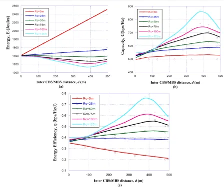
5.1. Effect of Inter-Cell Separation Distance

Figure 7. Behavior of: (a) capacity; (b) energy; (c) energy efficiency, energy efficiency vs. distance d for different

values of CBS radii .

due to increasing the available area for deploying this large number of CBSs (due to reduction of each cell’s coverage area). This will lead to more interferers to cause this capacity decay. The “turning point” that happens for different values of R_c and at different values of d, is found to cause

C

to act in a more sensitive way to varying R_c. Approaching the cell edge using CBS with larger coverage areas makes it more likely to find this turning point at larger d and vice versa. “The turning point” exists when Rc =25 m at d ≅380 m,

mean-while, it exists when Rc =100 m, at d≅440 m. Figure 7(b) shows the behavior of the model energy

con-sumption E when varying d for different values of R_c. It shows that for smaller values of R_c, the larger the d, the larger the E consumption (i.e. no energy is preserved).Energy consumption responds in a less sen-sitive way to d when R_c is increased to values of Rc =40 meters. Increasing Rc over 40 meters then will cause E to be more sensitive to increasing d and will cause energy consumption gain. A turning point from energy gain increase to decay of E is found to happen near the cell edges. Its location d depends on the val-ue of R_c. It is found that the best energy consumption (gain/preservation) occurs for Rc =125 m, d≅390 m. Figure 7(c), shows the behavior of Energy Efficiency

η

(bps/Hz/J) for different values of d (m) at several values of R_c (m). It is found that

η

increases with the increase of d till it inflects and starts decreasing due to the increase of deployable number of CBSs at a specific inter-MBS/CBS cell distance d (where

π

c c

N ≅ _ d R _). Energy efficiency

η

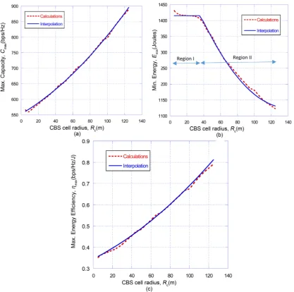
is more sensitive to the larger values of d, and larger values of R_c. Those peaks (maxima) found in the previously mentioned results happen at different situations depending on the values of d and R_c. This is tempting to investigate the behavior of those peaks (maxima). In another numeri-cal approach, the maxima of the obtained results are shown in Figure 8, the maximum values of

C

, E, and

η

c

[image:10.595.89.539.78.453.2]

η

were investigated by filtering maximum values of

C

, and plotting those maxima against the whole range of d and at different values of R_c in Figure 8(a). The results show that increasing R_c yields to an increase in maximum values of

C

(i.e. more radio resources per unit area). This is due to the increase in offloaded traffic from MBSs to CBSs, as a direct result of the increase of the covered area of CBSs. Figure 8(b) illustrates the case of filtering the minimum values of E obtained using the same method. Increasing the CBS cell radius will have small affect over the minimum values of energy consumption until near Rc ≅40 m. For bigger values

of R_c, it is found that minimum values of E will accomplish lower values, thus, more energy conservation will be achieved due to the reduction and saving in the RF power amplifications as well as the HVAC air condi-tion devices. Figure 8(c) illustrates the Energy Efficient Usage index

( )

η versus the CBS radius. It is found that increasing R_c will lead to an increase of the energy efficiency index, in addition, by increasing the CBS radius, there will be more energy saving (Figure 8(a)), and, gained throughput (Figure 8(b)).

5.2. Effect of CBS Coverage Area

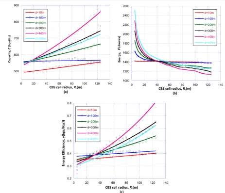
Figure 9(a) shows the behavior of capacity

C

against R_c for different values of d, The results show that

Figure 8. Shown in dotted red line, behavior ofmaxima: (a) capacity; (b) energy; (c) energy efficiency obtained for all values of inter MBS/CBSs distances versus CBS cell/coverage area radii Rc (shown in red dotted lines), and,

[image:11.595.92.510.265.679.2]

[image:12.595.74.538.78.476.2]

Figure 9. Behavior of: (a) capacity; (b) energy; (c) energy efficiency versus CBS cell/coverage area radii Rc for different values of distance d.

C

increases when increasing CBS cell radius, and it is more sensitive for larger values d, i.e. when CBSs are far away from MBS. For very small values of R_c, and since R_c is proportional to d, it is found that

C

is in its lowest value due to the inability of the system to offer more traffic offloading or additional resources. Figure 9(b) shows the behavior of E when varying d for different values of R_c. It shows that for smaller values of

c

R (<40 m), the smaller the d, the larger the E consumption, while, for this certain value of R_c (=40 m) energy consumption is the same for all CBS located at different locations away from MBS (all d). Also, the nearer the CBS to the MBS, the less sensitivity to varying the cell radius R_c. The figure also shows that for values of Rc>40 m, the larger the d, the lower the Energy consumption. This means that it is preferable to

use CBSs with larger values of R_c at the far distances from MBS, while for nearer distances it is preferable to use non-overlapping with smaller coverage CBS which will allow the usage of larger number of them, which in turn, will allow more traffic offloading opportunities.

Figure 9(c) shows the behavior of

η

against R_c for different d values. It shows that

η

increases with the increase of R_c, and it is more sensitive to larger values of d.

η

increases due to the increase of available number of CBSs deployed over the available d, where, as mentioned in the previous subsection:

π

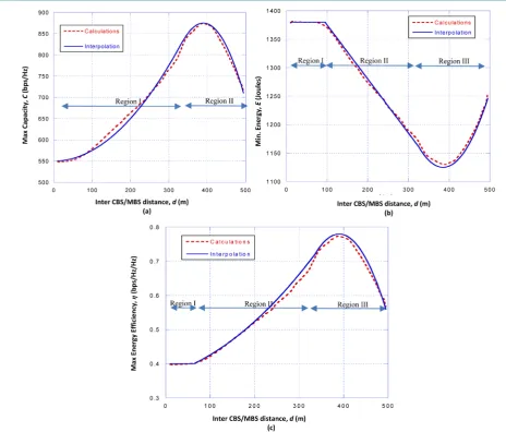
c c

[image:13.595.71.536.78.474.2]

Figure 10. Shown in dotted red line, maxima behavior of: (a) capacity; (b) energy; (c) energy efficiency versus distance d for different values of CBS cell/coverage area radii Rc.

mum obtained values of

C

, it is found that for nearer distances of d, capacity rises all the way till near the MBS cell edge, where it starts to inflict and decays again. Figure 10(b) shows the minimum consumed energy using different CBS cell radii, and for all the range of d. It follows an almost stable state near MBS, then it performs better energy consumption linearly all the range till near MBS cell edge (about 400 m) where it inflicts and starts to lose the ability to reduce energy consumption. These behaviors corporate in the behavior of

η

, where it is shown in Figure 10(c) that it starts to rise till near the MBS cell edge (about 400 m) where it inflicts and starts to decay.

5.3. Asymptotic Analysis

To reduce the complexity of calculations to find the asymptotic behavior of the previous results, deeper analysis is conducted. A mathematical reverse interpolation of the results is obtained. A unified formula is suggested to approximate these results. This is performed in order to provide a short but effective tool to help engineers working in the field of CR field planning. The suggested formula is applied with several parameters relative to the distance used (d or R_c). Because of the nonlinearity behavior of these results, a suggested form of a non-linear equation is used,

(

)

c

where a, b, c and d are the parameters used for results reverse interpolation. Moreover, because of the nonlinearity behavior of these results, results are dealt with as multiple regions’ curves, and apply different pa-rameters to each region.

It is found that the best parameters to fit the results’ interpolation are:

• maximum values of

C

, E, and

η

for different values of R_c:

(

)

2

max 0.009 c 85 480; 5 c 125,

C = R + + ≤R ≤ (Figure 8(a)) (21)

(

)

2

max

1415, ( , region I)

( , region II

5 36,

0.027 140 1125 36 125, )

c c c R E R R ≤ ≤ − + ≤ ≤  =   Figure 8(b)

Figure 8(b) (22)

(

)

2

5

max 1.15 10 Rc 95 0.23; 5 Rc 125,

η _{= ×} − _{+ + ≤ ≤ (Figure 8(c)) (23)}

• and, maximum values of

C

, E, and

η

for different values of d:

(

)

(

)

2

max 2

0.0023 5 560, 10 355,

0.015 390 860, 35

( , region I)

( , regi

5 50 ,0 on II)

d d C d d − + ≤ ≤ − + ≤  ≤  =   Figure 10(a) Figure 10(a) (24)

(

)

2

max

10 95, 95 325,

1380, ( , region I)

0.95 1470, ( , region II)

0.01 385 1125, 325 500 ( , region III)

d E d d d   = ≤ ≤ ≤ ≤ ≤ ≤ − +   − +  Figure 10(b) Figure 10(b) Figure 10(b) (25)

(

)

(

)

2 6 max 2 5 10 85,

1.8 10 97 0.35, 85 320

0.41, ( , region I)

( , region I ,

2 10 390 0.76 320 500

I)

( , region III)

d d d d d η − − ≤ ≤ × + + ≤ ≤ − ×   =    − + ≤ ≤ Figure 10(c) Figure 10(c) Figure 10(c) (26)

6. Conclusion

Using a combination of an analytical model and practical simulation, several outcomes have been achieved. Us-ing variable parameters of d (average distance between CBSs and MBS) and R_c (MBS coverage area radius), illustrated their effect on

C

(overall system capacity), and E (overall system energy consumption), and

η

(Energy Efficiency). When varying d, the results obtained show that increasing d will increase the overall system capacity

C

till near the edge of the MBS coverage, where

C

will start to decrease due to the decrease of the overall system SNR (due to the increase of the number of CBSs which will in turn increase the interfe-rence). Increasing d and using CBSs with cell radii of less than

<

40 m

will increase the system consump-tion of energy, while, with cell radii

>

40 m

will be a good choice for energy consumption saving policy. The more d approaches the MBS cell edge the more energy saving is obtained until an inflection point; where the system starts to reduce the energy saving. Finally the more d is increased the more

η

will be accomplished. Using CBSs with bigger cell radii will increase the sensitivity of

η

to respond to the effect of increasing d. When varying R_c, the results show that the overall system capacity

C

is more sensitive at larger d, while, the overall energy consumption E is more sensitive and inversely proportional to d at Rc<40 m and not

as sensitive and forwardly propotional to d at Rc >40 m. This indicates that using smaller non-overlapping

coverage area CBSs is preferable near the MBS. This work proposed several nonlinear equations with fixed coefficients to be used by field engineers to achieve the results by minimum reduced computation complexity.

References

[1] Correia, L.M., Zeller, D., Blume, O. and Ferling, Y. (2010) Challenges and Enabling Technologies for Energy Aware Mobile Radio Networks. IEEE Communications Magazine Special Issue on Green Radio, 48, 66-72.

http://dx.doi.org/10.1109/MCOM.2010.5621969

[2] ITU (2014) Energy Efficiency Metrics and Measurement Methods for Telecommunication Equipment L.1310, “Pre- Published Recommendations”. Telecommunication Standardization Sector of ITU.

Radio and Network. IEEE 20th International Symposium on Personal, Indoor and Mobile Radio Communications, Tokyo, 13-16 September 2009, 1-5. http://dx.doi.org/10.1109/pimrc.2009.5449938

[4] Hossain, E., Bhargava, V.K. and Fettw, G.P. (2012) Green Radio Communication Networks. Cambridge University Press, United Kingdom. http://dx.doi.org/10.1017/CBO9781139084284

[5] EARTH (Energy Aware Radio and Network Technologies—August 2014). EARTH.

https://www.ict-earth.eu/publications/deliverables/deliverables.html.

[6] Green Network Technologies INFSO-ICT-247733, Deliverable D3.2, EARTH.

https://bscw.ict-earth.eu/pub/bscw.cgi/d70460/EARTH_WP3_D3.2.pdf.

[7] FP7-ICT-2009-4-247733-EARTH Book (2012) EU Funded Research Project—January 2010 to June 2012, EARTH (Energy Aware Radio and Network Technologies). https://www.ict-earth.eu.

[8] FP7 in Brief (2014) Office for Official Publications of the European Communities, Luxembourg.

http://ec.europa.eu/research/fp7/pdf/fp7-inbrief_en.pdf.

[9] 7th Framework Programme for Research and Technological Development (2014) European Commission, Research & Innovation. http://ec.europa.eu/research/fp7/understanding/fp7inbrief/funding-schemes_en.html

[10] Magnus Olsson, E.A. (2012) A Methodology to Evaluate Radio Network Energy Efficiency at System Level. 1st ETSI TC EE Workshop, Genoa, Italy.

[11] TR 36.814, Further Advancements for E-UTRA Physical Layer Aspects RAN1 (2010) 3GPP in 2EPS.

http://www.in2eps.com/3g36/tk-3gpp-36-814.html.

[12] Auer, G., Giannini, V., Godor, I., Skillermark, P., Olsson, M., Imran, M.A., et al. (2011) Cellular Energy Efficiency Evaluation Framework. Proceedings of the IEEE 73rd Vehicular Technology Conference, Yokohama, 15-18 May 2011, 1-6. http://dx.doi.org/10.1109/VETECS.2011.5956750

[13] Gür, G., Bayhan, S. and Alagöz, F. (2013) Energy Efficiency Impact of Cognitive Femtocells in Heterogeneous Wire-less Networks. Proceedings of the 1st ACM Workshop on Cognitive Radio Architectures for Broadband—CRAB’13, Miami, 4 October 2013, 53-60. http://dx.doi.org/10.1145/2508478.2508480

[14] Bayhan, S. and Alagoz, F. (2012) Scheduling in Centralized Cognitive Radio Networks for Energy Efficiency. IEEE Transactions on Vehicular Technology, 62, 582-595. http://dx.doi.org/10.1109/TVT.2012.2225650

[15] Goldsmith, A. (2005) Wireless Communication. Cambridge University Press, Cambridge.

http://dx.doi.org/10.1017/CBO9780511841224

[16] Nandy, S.C. Voronoi Diagrams. Advanced Computing and Microelectronics Unit, Indian Statistical Institute, Kolkata 700108. http://www.tcs.tifr.res.in/~ghosh/subhas-lecture.pdf

[17] Miu, A. (2001) Lecture 7: Voronoi Diagrams. 6.838 Computational Geometry.

http://nms.lcs.mit.edu/~aklmiu/6.838/L7.pdf

[18] FP7 Project Management (2014) Eurescom Archive Website, July 2014.

http://archive.eurescom.eu/services/project_management/default.asp

[19] Abate, Z. (2009) WiMax RF Systems Engineering. Artech House, Boston and London.

[20] Gallager, R.G. (2001) Claude E. Shannon: A Retrospective on His Life, Work, and Impact. IEEE Transactions on In-formation Theory, 47, 2681-2695. http://dx.doi.org/10.1109/18.959253

[21] ETSI TR 136 913 V9.0.0, LTE; (2010-2012) Requirements for Further Advancements for Evolved Universal Terre-strial Radio Access (E-UTRA) (LTE-Advanced). Centre, 3GPP Mobile Competence.

[22] D6.13.7: Test Scenarios and Calibration Cases Issues 2. (2006) World Initiative New Radio (WINNER II), Deliverable, IST-4-027756.

[23] Requirements Related to Technical Performance for IMT-Advanced Radio Interface(s), M.2134, Report ITU-R. (2008).