Time Scale Approach to One Parameter Plane Motion by Complex Numbers

http://dx.doi.org/10.4236/apm.2015.51005

Time Scale Approach to One Parameter

Plane Motion by Complex Numbers

Hatice Kusak Samanci

1

_{, Ali Caliskan}

2

1_{Department of Mathematics, Faculty of Sciences, Bitlis Eren Üniversitesi, Bitlis, Turkey} 2_{Department of Mathematics, Faculty of Sciences, Ege Üniversitesi, Izmir, Turkey} Email: [email protected], [email protected]

Received 5 January 2015; revised 20 January 2015; accepted 23 January 2015

Copyright © 2015 by authors and Scientific Research Publishing Inc.

This work is licensed under the Creative Commons Attribution International License (CC BY). http://creativecommons.org/licenses/by/4.0/

Abstract

This paper presents building one-parameter motion by complex numbers on a time scale. Firstly, we assumed that E and E′ were moving in a fixed time scale complex plane and

{

0,e e1, 2

}

and

{

0 ,′ ′ ′e e₁, ₂

}

were their orthonormal frames, respectively. By using complex numbers, we

investi-gated the delta calculus equations of the motion on . Secondly, we gave the velocities and their union rule on the time scale. Finally, by using the delta-derivative, we got interesting results and theorems for the instantaneous rotation pole and the pole curves (trajectory). In kinematics, in-vestigating one-parameter motion by complex numbers is important for simplifying motion cal-culation. In this study, our aim is to obtain an equation of motion by using complex numbers on the time scale.

Keywords

Complex Numbers, Kinematic, Time Scales, Pole Curve

1. Introduction

The calculus on time scales was initiated by B. Aulbach and S. Hilger in order to create a theory that can unify discrete and continuous analysis, [1]. Some preliminary definitions and theorems about delta derivative can be found in the references [2]-[4].

In this study, some properties of motion in references [5]-[7] are investigated by using time scale complex planes. We find delta calculus equations of the motion and finally we get some results about the pole curves.

2. Preliminaries

Definition 2.1. Let  beanytimescale.Theforwardjumpoperator σ: → isdefinedby

( )

t : inf

{

s :s t

}

σ

= ∈ >

and the backward jump operator

ρ

: → is defined by

( )

t : sup

{

s :s t

}

, for t

ρ

= ∈ < ∈

In this definition, we put infΦ =sup (i.e.

σ

( )

t =t, if  has a maximum t) and supΦ =inf (i.e.

( )

t t

ρ

= , if  has a minimum t), where Φ denotes the empty set. If

σ

( )

t >t, we say that t is right-scat- tered, while if

ρ

( )

t <t we say that t is left-scattered. Points that are right-scattered and left-scattered at the same time are called isolated. Also if t<sup and

σ

( )

t =t, then t is called right-dense, and if t>inf and

( )

t t

ρ

= , then t is called left-dense. Points that are right-dense and left-dense at the same time are called dense. Finally, the graininess function

µ

:→

[

0,∞

)

is defined by

( )

: t t.

µ σ

= −

If f :→ is a function, then we define the function fσ :→ by

( )

(

( )

)

for all , . . .

fσ t = f σ t t∈ i e fσ = fσ

Let us define the interior of  relative to α which is a function that maps  into  to be the set

( )

( )

{

: either or and is not isolated

}

k

t α t t α t t t

= ∈ ≠ =

 

Definition 2.2. Assume f : → isafunctionandlet t∈k.Thenwedefine f∆

( )

t tobethenumber (pro- videditexists) withthepropertythatgivenanyε > 0, thereisaneighborhoodUoft (i.e. U = −

(

t

δ

,t+

δ

)

∩

forsome δ >0) suchthat

( )

(

)

( )

( ) ( )

( )

for all

f σ t f s f∆ t σ t s ε σ t s s U

 − − _ − _ ≤ − ∈

 

We call f∆

( )

t the delta (or Hilger) derivative of f at t. Moreover, we say that f is delta (or Hilger) differen-tiable on k provided f∆

( )

t exists for all k

t∈ .

Theorem 2.1. Assume f :→ isafunctionandlet k

t∈ .Thenwehavethefollowing: 1) If f is differentiable at t, then f is continuous at t.

2) If f is continuous at t and t is right-scattered, then f is differentiable at t with

( )

f

(

( )

t

_{( )}

)

f t

( )

f t

t

σ µ

∆ ₌ −

3) If t is right-dense, then f is differential at t if the limit

( )

( )

lim_{s t} f t f s

t s

→

− −

exists as a finite number. In this case a given

( )

lims t

( )

( )

f t f s f t

t s

∆

→

− =

− 4) If f is differentiable at t then

( )

(

)

( )

( ) ( )

f σ t = f t +µ t f∆ t

Theorem 2.2. Assume f g, :→ aredifferentiableat t∈k.Then: 1) The sum f +g:→ is differentiable at t with

2) For any constant, α α, f :→ is differentiable at t with

( ) ( )

αf ∆ t =αf∆

( )

t

3) The product fg:→ is differentiable at t with

( ) ( )

fg ∆ t =f∆

( ) ( )

t g t +f

(

σ

( )

t

)

g∆

( ) ( ) ( )

t =f t g∆ t +f∆

( )

t g

(

σ

( )

t

)

4) If f t f

( )

(

σ

( )

t

)

≠0 then 1

f is differentiable at t with

( )

_{( )}

₍

( )

_{( )}

₎

1 f t

t

f f t f σ t

∆ _∆

  _{= −}    

5) If g t g

( )

(

σ

( )

t

)

≠0, then f

g is differentiable at t with

( )

f

( ) ( )

t g t

_{( )}

₍

f t g

_{( )}

( ) ( )

₎

t f

t

g g t g σ t

∆ _{∆ ∆}

−

  ₌

   

In the reference [3], the chain rule on time scales is given for various cases.

Theorem 2.3. Assume g:→ iscontinuous, g:→ isdeltadifferentiableon k_{, and}

:

f →

iscontinuouslydifferentiable.Then, thereexists c intherealinterval _t,σ

( )

t _ with

(

f g

) ( )

∆ t = f′

(

g c

( )

)

g∆

( )

t

Theorem 2.4. Let f :→ becontinuouslydifferentiableandsuppose g:→ isdeltadifferentiable. Then f g:→ isdeltadifferentiableandtheformula

(

) ( )

{

1

(

( )

)

( ) ( )

}

( )

0

= d

f g ∆ t

∫

f′ g t +hµ t g∆ t h g∆ t

holds.

Theorem 2.5. Assume that v:→ is strictly increasing function and :=v

( )

 is a time scale. Let

:

w  →.If v∆

( )

t and w∆

( )

v t

( )

existfor t∈k, then

(

w v

)

∆ =

(

w∆v v

)

∆ (2.1)

Definition 2.3. Forthegiventimescales ₁ and ₂, letusset

{

}

1+i 2= z= +x i :y x∈ 1,y∈ 2

    (2.2)

where i= −1 is the imaginary unit. The set  ₁+i ₂ is called the time scale complex plane. Definition 2.4. For h>0, wedefinethecylindertransformation ξh:h→h by

( )

1

(

)

= Log 1

h z zh

h

ξ +

and for h=0, let ₀:=.

Definition 2.5. If p∈, thenwedefinetheexponentialfunctionby

( )

, exp

(

( )

(

( )

)

)

for ,

t

p _s

e t s =

∫

ξ_{µ τ} p τ ∆τ s t∈

1) e t s₀

( )

, ≡1 and ep

( )

t t, ≡1;

2) e_p

(

σ

( )

t ,s

)

= +

(

1 µ

( ) ( )

t p t

)

e_p

( )

t s, ;

3)

( )

1, p ,

p

e t s e t s =  ;

4)

( )

( )

1

( )

, ,

,

p p

p

e t s e s t

e s t

= = _ ;

5) ep

( ) ( )

t s e, p s r, =ep

( )

t r, ;

6) ep

( ) ( )

t s e t s, q , =ep⊕q

( )

t s, ;

7)

( )

( )

( )

,

, ,

p

p q q

e t s

e t s

e t s =  ;

8)

( )

( )

( )

1

, ,

p p

p t

e t s eσ t s

∆

 

= −

 

 

  ;

Theorem 2.7. Assume

σ

( )

t >t for t∈κ

( )

,0

( ) ( )

,0

p p

e∆ t t = p t e t t Theorem 2.8. If p q, ∈h then

( ) (

) ( )

_{( )}

0 0

0

, ,

,

p p q

q

e t t

e t t p q

eσ t t

∆ _{= −}



Theorem 2.9. If p∈_h and a b c, , ∈ then

( )

,

( )

,

p p

e c s ∆ p e c s σ

  = −  

   

3. One Parameter Motion and Hilger Complex Numbers on a Time Scale

Assume that  is a time scale. Let us set the time scale complex plane for as

{

}

i z x i :y x ,y + = = + ∈ ∈

 (3.1)

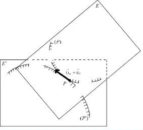
Here, let E and E′ be moving in a fixed time scale complex plane. The motion is called as one-parameter planar motion by the complex numbers on the time scale and denoted as H₁=E E′ for a planar motion of E

relative to E′.

{

0, ,e e_{1 2}

}

and

{

0 , ,′ ′ ′e e_{1 2}

}

be their orthonormal frames, respectively. We suppose that

{

0 , ,′ ′ ′e e_{1 2}

}

is fixed, then we say that

{

0, ,e e_{1 2}

}

moves with respect to

{

0 , ,′ ′ ′e e_{1 2}

}

, e_i,

(

i=1, 2

)

are the functions of a time scale parameter t. Let x=

(

x x₁, ₂

)

and x′=

(

x x₁′ ′, ₂

)

be the position vectors of a point X in the plane, as following we can write the coordinates of the point X by using complex numbers on the time scale with respect to a fixed or moving plane E and E′, respectively. So:

1 i 2 and 1 i 2

x x ′ x′ x′

= + = +

x x

The translation vector O O′ can be written as the following equation on a fixed plane E′:

1 i 2

u′ u′ = +

u

by using the definition of the time scale complex plane. The translation vector is more suitable as

1 i 2

OO′ u u

== − −

u

for doing the formulas symmetric on the moving plane.

*

x′



Figure 1. One parameter planar motion on time scale.

( )

, 0

(

i

( )

)

p

e t t ϕ t

 

= −   

u u (3.2)

For any point X, the vector x′ is

( )

, 0

(

i

( )

)

p

e t t ϕ t

 

′= ′_{+   }

x u x (3.3)

By substituting u′ in the Equation (3.3)

( )

, 0

(

i

( )

)

( )

,0

(

i

( )

)

p p

e t t ϕ t e t t ϕ t

   

′ = − _{  }+ _{  }

x u x

(

)

ep

( )

t t, 0

(

iϕ

( )

t

)



′ = − + _{  }

x u x (3.4)

Then, we can obtain the vector x as follows:

( )

(

( )

)

( )

0

(

( )

)

0

, i

, i p

p

e t t t

e t t ϕ t ϕ

′

 

′

= + _{= +  }

 

   

x

x u u x _

Here, assume the functions

( )

t , ′

( )

t ,

ϕ ϕ

( )

t

= = =

u u u u

are ∆-differentiable functions and the parameter t is defined as t₀≤ ≤t t₁ on the  time scale. We will cal- culate the formulas for a fixed or moving plane.

Definition 3.1. Avelocityvector ofthepointXwithrespect toEiscalled ∆-relativevelocityvectorofthe pointXonthetimescale.Theequationofrelative ∆-velocityvectoris

d

r

t

∆

∆ = _∆ =

x

x x (3.5)

Definition 3.2. Avelocityvector ofthepointX withrespect toEiscalled ∆-relativevelocityvectorofthe pointXonthetimescale.Theequationoftherelative ∆-velocityvectoris

( )

,0

(

i

( )

)

r r ep t t ϕ t

∆′ = ∆   

x x (3.6)

( )

,0

(

i

( )

)

p

e t t ϕ t

∆_{ }

=x _  _ (3.7)

for the fixed time scale complex plane.

Definition 3.3. A velocityvector of the point X with respect to the time scale complex plane E′ on the planarmotion H_I =E E′ whichbelongstoacurve

( )

X′ ofthepoint X′ on E′ iscalledthe ∆-absolute velocityvectorofthepointXonthetimescaleandisdenotedby x_∆a.

Definition 3.4. On the planar motion H_I =E E′, while the point X is fixed on the moving time scale complexplane E (i.e. x_∆r =0), a velocityvectorofthepointXiscalledthe ∆-draggingvelocityvectorof thispointonthetimescaleandisdenotedby x_∆f .

So, we obtain the ∆-absolute velocity x_∆a, i.e. the velocity of X with respect to the plane E′, from the Equation (3.4) using Equation (3.2).

(

) ( )

(

( )

)

{

}

( )

(

( )

)

( )

(

( )

)

{

}

( )

(

( )

)

{

}

( )

(

( )

)

( )

(

( )

)

0 0 0 0 0 0 d , i

, i , i

, i

, i , i

a p

p p

p

p p

e t t t

t

e t t t e t t t

e t t t

e t t t σ e t t t

ϕ ϕ ϕ ϕ ϕ ϕ ∆ ∆ ∆ ∆ ∆ ∆ ∆ ∆ ′   ′ = = = − + _{ } ∆     = − _{ }+ _{ }   ′ = _{+  }     ′ = + _{ }+ _{ }       x

x x u x

u x

u x

u x x

( )

,0

(

i

( )

)

( )

, 0

(

i

( )

)

i

( )

.

p p

e t t ϕ t σ e t t ϕ t ϕ t

∆ ∆_{  } ∆ _ ∆

′

=u +x _  _+x _   _

by Theorem 2.5. Also

( )

,0

(

i

( )

)

( )

,0

(

i

( )

)

i

( )

a ep t t t ep t t t t

σ

ϕ ϕ ϕ

∆ ∆ ∆ ∆

∆′ =   + ′ + _   _

x x u x

and using Theorem 2.7, we have

( )

,0

(

i

( )

)

( )

,0

(

i

( )

)

i

( )

a ep t t t pep t t t t

σ

ϕ ϕ ϕ

∆ ∆ ∆

∆    

′ = _{  }+ ′ + _{  }

x x u x

Here,

ϕ

∆ is called a delta-angular velocity of the motion H_I on a time scale, and remembering Equations (3.3) and (3.7), we can find the dragging velocity vector x_∆f of the point X

( )

( )

0

(

( )

)

i , i

f t p ep t t t

σ

ϕ ϕ

∆ ∆

∆ = ′ +  ⋅  

x u x (3.8)

( )

(

)

ipϕ t σ σ

∆ ∆

′ ′ ′

=u + x −u (3.9)

with the restriction

ϕ

∆≠0, from Equation (3.2) by taking the ∆-derivative with respect to the parameter t, we get the following equation.

( )

(

( )

)

( )

(

( )

)

( )

(

( )

)

( )

(

( )

)

( )

(

( )

)

( )

( )

(

( )

)

( )

(

( )

)

( )

( )

(

( )

)

( )

( )

(

( )

)

0 0 0 0 0 0 0 0 0 , i

, i , i

, i , i i

, i , i i

, i i , i .

p

p p

p p

p p

p p

u e t t t

e t t t e t t t

e t t t e t t t t

e t t t pe t t t t

e t t t p t e t t t

σ σ σ σ ϕ ϕ ϕ

ϕ ϕ ϕ

ϕ ϕ ϕ

ϕ ϕ ϕ

∆ ∆ ∆ ∆ ∆ ∆ ∆ ∆ ∆ ∆ ∆   ′ = −_{ }     = − _{ }− _{ }     = − _{ }− _{ }     = − _{ }− _{ }     = − _{ }− _{ }           u u u u u u u u u

( )

, 0

(

i

( )

)

i

( )

p

u′∆ = −u∆_e t t  ϕ t _+ pϕ∆ t u′σ (3.10)

Theorem 3.1. A ∆-absolutevelocityvectorisequaltoaddinga ∆-relativevelocityvectorand ∆-dragging velocityvectoronthemotion H_I =E E′, i.e.

a f r

x_∆ =x_∆ +x_∆ (3.11)

Proof. By using Equation (3.10) and Equation (3.5), we can get the following equations:

( )

(

( )

)

( )

(

( )

)

( )

(

( )

)

( )

{

}

( )

(

( )

)

( )

(

( )

)

( )

0

0 0 0

0

, i

, i , i i , i

, i i

.

a a p

p p p

p

r f

e t t t

e t t t pe t t t t e t t t

e t t t p t

σ

σ

ϕ

ϕ ϕ ϕ ϕ

ϕ ϕ ∆ ∆ ∆ ∆ ∆ ∆ ∆ ∆ ∆   ′ = _{ }   ′     = _{ }+ + _{   }   ′ = + _{ }+ = +      x x

x u x

x u x

x x







and thus, we get the relation of the velocities:

a r r

∆ = ∆ + ∆

x x x

We have

( )

, 0

(

i

( )

)

f f e p t t ϕ t

∆ = ∆′   

x x _

We will calculate x_∆f here using Equation (3.9) and Equation (3.10);

( )

(

)

{

}

( )

(

( )

)

( )

(

( )

)

( )

(

)

( )

(

( )

)

( )

(

( )

)

( )

{

}

( )

(

( )

)

( )

{

( )

(

( )

)

( )

}

( )

(

( )

)

0 0 0 0 0 0 0

i , i

, i i , i

, i i , i

i , i i , i

f p

p p

p p

p p

u p t u e t t t

u e t t t p t u e t t t

e t t t p t e t t t

p t e t t t p t e t t t

σ σ

σ σ

σ

σ σ

ϕ ϕ

ϕ ϕ ϕ

ϕ ϕ ϕ

ϕ ϕ ϕ ϕ

∆ ∆ ∆ ∆ ∆ ∆ ∆ ∆ ∆ ∆   ′ ′ ′ = + − _{ }     ′ ′ ′ = _{ }+ − _{ }   ′   = − _{ }+ _{ }     ′ ′ + _{ }− _{ } = −        x x x u u x u u      

( )

( )

0

(

( )

)

ip t e p t t, i t .

σ

ϕ∆ _{′ } ϕ _

+ x _{ }  _

and

( )

(

)

i

f p t

σ σ

ϕ

∆ ∆

∆ = − + −

x u x u (3.12)

Theorem 3.2. Thereisonly onepointatwhichthe ∆-dragging velocityiszeroforanyinstant t∈, i.e. whichisfixedonthebothoftheplanes E and E′, withtherestriction

ϕ

∆≠0 onthemotion H_I =E E′.

Proof. The points at which the ∆-dragging velocity vector is zero for any instant t∈ have to stay fixed for not only the plane E, but also for the plane E′ on the motion H_I =E E′. By taking x_∆f =x_∆′_f =0 for fixed and moving planes, from (3.15) and (3.8):

( )

(

)

i 0

f p t

σ σ

ϕ

∆ ∆

∆ = − + − =

x u x u (3.13)

( )

(

)

i 0

f p t

σ σ

ϕ

∆ ∆

∆′ = ′ + ′ − ′ =

x u x u (3.14)

we can obtain the following complex vectors;

( )

i

P

p t

σ σ σ

ϕ ∆

∆

= = + u

x u (3.15)

( )

i

P

p t

σ σ σ

ϕ ∆

∆ ′ ′ = ′ = ′ − u

which are given σ -instantaneous rotation pole P on both coordinate systems. Because, the affine axioms Pσ, P′σ are the end-points of Xσ, X′σ, respectively.

Definition 3.5. Thepoint Pσ whichcorresponds to the position vector Pσ =

(

p₁σ,p₂σ

)

is calledthe for- wardpoleortheinstantaneous rotationpoleortheinstantaneous rotationcenterforthemovingplane onthe timescalemotion H_I, inFigure 2.

Definition 3.6. Thepoint P′σ whichcorrespondstothepositionvector P′σ =

(

p₁′σ,p₂′σ

)

iscalledthefor- wardpoleortheinstantaneousrotationpoleortheinstantaneousrotationcenterforthefixedplaneonthetime scalemotion H_I, inFigure 2.

We can get the following equations from Equation (3.15) and Equation (3.16):

( )

(

)

ipϕ t σ σ

∆ ₌ ∆ ₋

u P u (3.17)

( )

(

)

ipϕ t σ σ

∆ ∆

′ = − ′ − ′

u P u (3.18)

By eliminating u∆ and u′∆ from Equation (3.13) and Equation (3.14), the dragging velocity becomes as following:

( )

(

)

i

f p t

σ σ

ϕ∆

∆ = −

x x P (3.19)

( )

ipϕ∆ t σ σ

= P x (3.20)

and;

( )

(

)

( )

i

i .

f p t

p t

σ σ

σ σ

ϕ ϕ ∆ ∆

∆

′ = ′ − ′

′ ′ =

x x P

P x

4. Conclusions

[image:8.595.174.457.449.707.2]

Result 4.1. Tworesultsforthe ∆-draggingvelocityofthe point X onthe movingplanecanbeobtained as follows:

1) Since scalar product of the vector is

(

x1 p1

) (

i x2 p2

)

σ σ ₌ σ ₋ σ ₊ σ ₋ σ

P X

and the vector x_∆f is zero, these vectors are perpendicular. 2) The length of the vector x_f can be calculated as follows:

(

) (

2

)

2

1 1 2 2

f x p x p p p

σ σ σ σ _ϕ∆ σ σ _ϕ∆

∆ = − + − =

x P X

here P Xσ σ denotes for the length of P Xσ σ. From this result, we get the following theorem:

Theorem 4.1. On the motion H_I, the pointsX ofthe moving plane Edraw trajectories onthe fixed time scalecomplex plane E′ which their normals (trajectory normals) passfrom the instantaneousrotation pole

Pσ.

Theorem 4.2. EverypointofXofthemovingplaneEisdoingrotationalmovement (instantaneousrotation movement) witha Pσ-centered,

ϕ

∆-angularvelocityandpfactoroninstantt.

Since X is an arbitrary point of the time scale complex plane E, we can give the following theorem:

Theorem 4.3. Aone-parametermotionconsists ofrotation with

ϕ

∆ angularvelocityandp factoraround theinstantaneousrotationpole Pσ ofthemovingplaneEontinstant, i.e.theplane Erotateswiththe angle

ϕ

∆

andthefactorparoundthepoint Pσ onthetimeelement ∆t.

Theorem 4.4. Thevelocity vectors ofthe instantaneous rotation pole Pσ which draws the forward pole curvesonthemovingandfixedplanesisthesamevectorateachinstantt.

Theorem 4.5. Onone-parameterplanarmotion H_I themovingpolecurve

( )

Pσ oftheplaneErollsonto thefixedpolecurve

( )

P′σ oftheplane E′ withoutsliding.

Result 4.2. Withoutbeingdependedontime, amotion H_I occursbyrolling, withoutsliding, thecurve

( )

P

ofEontothecurve

( )

P′ of E′.

References

[1] Aulbach, B. and Hilger, S. (1990) Linear Dynamic Processes within Homogeneous Time Scale. Nonlinear Dynamics and Quantum Dynamical System, Berlin Akademie Verlag, 9-20.

[2] Bohner, M. and Peterson, A. (2003) Advances in Dynamic Equations on Time Scales, Birkh a _User.

[3] Bohner, M. and Peterson, A. (2001) Dynamic Equations on Time Scales, An Introduction with Applications, Birkh a User.

[4] Bohner, M. and Guseyinov, G. (2005) An introduction to Complex Functions on Products of Two Time Scales. Jour-nal of Difference Equations and Applications, 12.

[5] Bottema, O. and Roth, B. (1990) Theoretical Kinematics. Dover Publications, Mineola.