Use of regression trees in the study of nonparametric wage structures

(1)

Use of regression trees in the study

of nonparametric wage structures

by

Ricardo Mora

Thesis submitted for the degree of doctor of Philosophy (PhD) on February, 1998

at

(2)

INFORMATION TO ALL USERS

The quality of this reproduction is dependent upon the quality of the copy submitted.

In the unlikely event that the author did not send a complete manuscript and there are missing pages, these will be noted. Also, if material had to be removed,

a note will indicate the deletion.

Dissertation Publishing

UMI U615554

Published by ProQuest LLC 2014. Copyright in the Dissertation held by the Author. Microform Edition © ProQuest LLC.

ProQuest LLC

789 East Eisenhower Parkway P.O. Box 1346

(3)

IH£SC

S

F

(4)

My foremost thanks are due to Danny Quah for his supervision and encouragement over the last four years. My thanks should also go to Irini Moustaki and Pedro Delicado not only for their advice and helpful comments but also for their kind readiness to help whenever asked. I want to express my thanks to all members of the Economics Department at the London School of Economics where I have found a very friendly and encouraging environment. Financial

support from the Bank of Spain is also greatly acknowledged.

(5)

Abstract

This study is concerned with the application of multivariate

nonparametric models known as regression trees to the analysis of the

U.S. wage structure. In Chapter 1, I first review regression trees and

other available multivariate nonparametric techniques, highlighting

their differences and common features. In the second part of Chapter 1,

I look at the literature on the U.S. wage structure in connection with

the issue of functional specification and argue that regression trees

is particularly well suited for analyzing wage structures. In Chapter

2, I implement regression trees on U.S. wages for white male workers to

estimate experience-wage profiles and unveil local sudden breaks in the

profiles at the end of the working life. For 1980, these breaks account

for about 50% of the negative average differential between the last two

experience groups. This effect decreases continuously until 1995. In

Chapter 3 I propose a simple extension of the Oaxaca-type average wage

gap decompositions between any two groups of workers. This procedure

can be carried out without any compromise in the interpretation using

a nonparametric wage structure. I then study wage gap decompositions

for Mexican workers in the U.S. labor market. Finally, in Chapter 4 I

apply regression trees to study both the relative growth performance of

workers' real wages and the sources of wage dispersion and its

evolution in the U.S. from 1980 onwards. On trends, the technique

uncovers a linear structure for the growth experience of white workers

with less than forty years of experience. On dispersion, at least 10%

of the increase in observed variance came from changes in the structure

(6)

page

Acknowledgements 2

Abstract 3

Contents 4

List of tables 7

List of figures 9

1 Introduction:

Regression

trees and nonparametric

wage structures

12

1.1 Regression trees and predictive learning 12 1.1.1 Least squares parametric regression 18 1.1.2 Single hidden layer artificial neural

networks 19

1.1.3 Projection pursuit and multiple hidden

layer artificial neural networks 22

1.1.4 Tree structures 23

1.1.5 Universal approximators 25

1.2 Estimation of regression trees 26

1.3 Regression trees in economics 34

1.3.1 A classification algorithm 34

1.3.2 Melon prices 36

1.3.3 Multiple growth regimes 37

1.4 Nonparametric Wage Structures 39

1.4.1 Wage structures 39

(7)

2 Tree estimation of experience-wage profiles

59

2.1 Introduction 59

2.2 The theoretical framework 62

2.2.1 Ben-Porath (1967) 66

2.2.2 Uncertainty and human capital 74 2.2.3 A simple model of uncertainty in the

depreciation of human capital 75

2.3 The econometric model 81

2.4 Empirical results 85

2.5 Conclusions 103

Appendix A 105

Appendix B 112

3 Decomposition of average

wage differentials for

nonparametric wage structures: An application

to Mexican workers in the

U.S.

114

3.1 Introduction 114

(8)

3.2.1 The parametric approach 116 3.2.2 Nonparametric decompositions 121

3.3 Empirical findings 124

3.3.1 Parametric and nonparametric average wage gap decompositions for workers of

Mexican origin 124

3.3.2 Average non-Hispanic-Mexican wage

differentials in the border states 137

3.4 Conclusions 141

Appendix C 154

An application of regression trees to the

analysis of the evolution of the U.S. wage

structure since 1980

155

4.1 Introduction: Relative growth performance

and dispersion changes in wages 155

4.2 Random fields and dynamic wage structures 158

4.2.1 Dynamic wage structures 158

4.2.2 A dynamic index model for dynamic

wage structures 160

4.3 A review of trend estimators 166

4.4 Trends in U.S. real wages 171

(9)

Contents

4.4.2 Empirical results 175

4.5 Wage dispersion and nonparametric dynamic

wage structures 181

4.6 Conclusions 190

Appendix C 199

5

Conclusions

209

(10)

2.1 Goodness-of-fit results for logwage regressions.

Human capital specification 89

2.2 Experience wage differentials in the nonparametric

surfaces and vintage effects 93

2.3 General breaks in accumulation paths and experience profiles 95 2.4 Parametric specification searches for each type of

worker along the nonparametric surfaces 97 2.5 Tests for sudden losses of human capital 100 2.6 Effects on average wages at each level of experience

of human capital 102

2.7 No. of observations in each cell. 1980 110 2.8 No. of observations in each cell. 1985 110 2.9 No. of observations in each cell. 1990 111 2.10 No. of observations in each cell. 1995 111 3.1 Regression results: Goodness-of-fit measures for

the Mex data set 124

3.2 Average wage decompositions. Mex data. Reference variable: Country of birth. Reference worker: born

in Mexico 133

3.3 Average wage decompositions. Mex data. Reference

variable: Ethnic. Reference worker: Mexicano 136 3.4 Average Wage Decompositions. Texmex data. Reference

variable: Ethnicity. Reference worker: Mexican

(11)

Liat of

4.1 Main growth experiences from regression trees. Latent growth indicator. Trends data.1980-1995

4.2 Growth structure for white workers with less than 40 years of experience. Trends data

4.3 Regression trees: Validation results. Dispersion data. 1980-1995

4.4 Wages and tree residuals. Dispersion data. Basic statistics

4.5 The effect of structural change in observed wages dispersion. Dispersion data.1980-1995

4.6 The effect of structural change. Correlation matrix. Dispersion data.1980-1995

4.7 Simulation results

tabl«s

179

181

184

186

187

(12)

1.1 2D representation of structure f(x1#x2) 55 1.2 Binary tree representation of structure f(x1/x2) 56 1.3 Binary tree representation of a 4-dimensional tree

structure 57

1.4 2D representation of a general tree structure 58 2.1 Average wages of white, male, nonfarm, full-time

employed workers 105

2.2 Experience-wage profiles. Unweighted averages of

nonparametric projections. 1980 106

3.1 Average residual sum of squares for the sequence of

optimal subtrees .Estimation and Test Samples. Mex data 147

3.2 Tree T21. Mex data 148

3.3 Wage differentials projected by T21 between workers born in the U.S. and workers b o m in Mexico 149 3.4 Wage differentials projected by T21 between

Mexican-Americans and Mexicanos 150

3.5 Residual sum of squares for the sequence of optimal

subtrees. Test Sample. Texmex data 151

(13)

List of figurss

3.7 Wage differentials projected by T8 between Mexican and White Nonhispanic

4.1 Latent growth indicator vs average rates. Trends data Estimation sample. 1980-1995

4.2 Latent growth indicators vs average rates. Trends data Test sample.1980-1995

4.3 Histogram for latent growth indicator. Trends data. Estimation sample. 1980-1995

4.4 Histogram for latent growth indicator. Trends data. Test sample. 1980-1995

4.5 Residual sum of squares for the sequence of optimal trees. Trends data. Latent growth estimator

4.6 Tree T182. Trends data

4.7 Histogram for regression tree test sample residuals. Dispersion data. 1980

153

199

200

201

202

203 204

205

206

207

(14)

Introduction: Regression trees and nonparametric

wage structures

In the following chapters I will be concerned with the

application of multivariate nonparametric models known as

regression trees to the analysis of the U.S. wage structure. In

this chapter, I first review neural networks, projection pursuit

and regression trees -all of them available multivariate

nonparametric techniques-. Then, I present a brief survey on

empirical results on the wage structure in the U.S. labor

market. The chapter ends with an outline of the rest of the

thesis.

1.1 Regression trees and predictive learning

Mathematics, statistics, engineering, artificial intelligence,

(15)

Chapter 1: Introduction

learning. A simple example of a predictive learning problem

involves one set of variables, sometimes called inputs,

sometimes called explanatory variables, and other times called

independent variables, and just one variable called either

output, response, or dependent variable. This variable is

defined over a subset of the real line1.

The problem can consist of designing a system with which

interpolations of the output can be obtained from the inputs.

This is a mathematical problem called function approximation.

If some of the inputs are not observable, the mathematical model

is of a statistical nature. Let the model be

y = f ( x 1 , • • • ,xn) + e = f (x) + e. (1.1)

In (1.1) I assume an additive relation for the two sets of

independent variables. The residual e is the effect of all the

unobserved variables on the dependent variable. A fixed effect

can be thought both as an observed constant effect and as the

effect of a constant unobserved variable. This makes model (1.1)

ambiguous. To solve this ambiguity, the unobserved residual e

can be defined by E[e|x]=0 where E[] is the expectation

operator.

The objective of predictive learning is to obtain a useful

1 In statistics, when the response is categorical, the

(16)

approximation to f(x)=E[y|x].

Neural networks use finite learning samples {yi/X^ and learning

algorithms to produce outputs f* in response to inputs x* and

adapt its outputs f* according to residuals { (yi-f*(Xi) ) }iB

Statistics seeks to obtain true approximations of f on the local

area defined by the finite sample {y^x.^. Thus, the stress in

statistics is on validating results while the stress in neural

networks is on learning.

Predictive learning is implemented through an optimization

problem on a finite sample. The objective function could be

An infinite number of functions can yield the minimum value,

zero, for the solution in (1.2). In order to obtain a well

defined problem in finite samples2, further assumptions must be

2 The similar problem for a "sample of infinite size" is

well defined in the sense that only f (•) will be the solution

of the problem. Thus,

f (x) (1 .2 )

f (x)

g

+ e - g (x) ] 2 p (x) dx.

(17)

Chapter 1: Introduction

added. Every predictive learning method can be characterized as

a set of constraints on problem (1.2).

There are two general forms of restrictions. The first way to

restrict the problem is to place constraints on the class of

eligible functions g(x). The second alternative consists of

selecting a small number of input variables, so that the

dimension of the variable space is small relative to the finite

sample.

For high dimensional spaces, the second alternative is in many

practical cases not feasible. The reasons are generally known

as the curse of dimensionality. Firstly, there is the problem

of minimum required number of observations to have a densely

packed sample. If 100 observations represents a dense sample for

a single input system, then for xeRN, the required sample would

be 100N. For 10 input variables we would need 1020 observations.

Secondly, all observations are close to an edge of the sample3.

Consider a sample of three observations in a one-dimensional

problem. Two of the observations must be at the edge of the

sample. If you add a new dimension (input) to the problem, all

three observations will be at the edge, making interpolation

impossible.

3 That is, there are no more observations between that

(18)

The only way to overcome these problems in a high dimensional

setup is by incorporating outside knowledge -knowledge not

related to the sample- in the way of functional restrictions.

A direct way of doing this is by incorporating a penalty to

criterion (1.2):

The best penalty <p>0 is one that has small values for those g(x)

that are close to f (x) and large values otherwise. The strength

parameter A is inserted so that the penalty effect can be

adjusted independently from its form.

If no restriction is imposed on A, then we might want to solve

the two-step problem:

However, this is not very interesting since (1.4) always yields

The best fit is given by the solution without penalty. This fit,

however, may be very poor for any other independent sample,

i.e., the estimated surface may have very low predictive power.

A common approach to overcome overfitting is to divide the

sample into a learning and a test sample. The learning sample

f (x) (1.3)

(1.4)

(19)

Chapter 1: Introduction

pursuit, neural networks, and regression trees5. The objective

is to highlight what is common between these methods and what

characterizes regression trees more neatly.

1.1.1 Least squares parametric regression

Penalty function 0 takes the form

where h(*) is a continuous, doubly differentiable function with

respect to 8 that is completely specified but for a finite

number of unknown parameters in 0.

Problem (1.3) collapses to

The choice of A becomes irrelevant and there is no need for

cross-validation.

5 For an introduction of neural networks, see e.g. Kuan and

White (1994). See Huber (1984) for a review on projection

pursuit. The basic reference for regression trees is Breiman et

alia (1984). These are the most popular predictive learning

models.

<t> [g (x) ] = - if g(x) + h(x | 01,...,8k)

4>

[g

(x) ] = 0 if g (x) = h(x I 0lf . . ., 0k) , (1.6)

= argmin 0x e*

(20)

Assuming certain statistical properties for the error term, e,

leads to a complete inferential theory.

The function h(*) needs not be linear, as it is the case of the

binary logit probability model, where

h(x | 9) = G (x, 0) = --- ---- -— . (1.8)

1 + exp (-x 6)

This is a multivariate nonlinear model and can be thought of as

a three-layer system. The first layer corresponds to the inputs,

x. The second layer is the linear index of the inputs, x' 0. The

third layer is the output h(*).

The model is flexible in the sense of giving nonlinear responses

because of the nonlinear relation between the second and the

third layer. This fundamental source of flexibility is fully

exploited in artificial neural networks, projection pursuit, and

regression trees.

1.1.2 Single hidden layer artificial neural networks

Penalty function <p now takes the form

<J>[g(x) ] = °° if g(x) f J h T(x | 0) J (19)

<t>Cg(3c)] = p(9)< 00 else

(21)

Chapter 1: Introduction

h (x|a,y) = ]fcat ’ s( x V t ) (1.10)

t-i

and s(*) is any smooth sigmoid function such that 0£s(*)£l

Thus, G(*) in (1.8) is one of such functions6.

The indicator function

1 if p true

I(li) = (1.11)

0 if p false

was chosen as s (• ) in the first published articles on neural

networks. The indicator function is an activation devise. It

incorporates a new structure to model (1.10) when a threshold

is overcome in an index or hidden layer.

For some applications, smooth functions as activation devices

seem more useful than step functions. In biological neural

systems there is a tendency of certain types of neurons to be

idle in the presence of low levels of observed input activity,

and to become active only after input activity passes a

threshold. However, in empirical studies the threshold cannot

Another common example is the arctangent function:

1 _ -l 1 s (z) = — tan z + — .

(22)

be properly detected when the problem is highly complex, as when

there are millions of switches. Therefore, it is probably a

better modelling strategy to bet on smooth activation functions,

where the threshold is blurred.

There are three ways in which (1.10) generalizes over (1.8).

Although model (1.10) has also three layers, its second layer

is more complex than the second layer in model (1.8). This layer

is usually called the hidden layer in the neural network

literature. The number of elements in the hidden layer is not

fixed to one, but chosen in the optimization. The second way in

which model (1.10) is more general is that each component of the

second layer affects the output independently. The extent to

which it does so, am, must also be estimated. The smooth

activation function, s (•), can be chosen from several

alternatives. Finally, cross-validation is crucial and the

selection of p ( ‘ ) will influence the complexity of the

estimated model.

The role of s (• ) is pivotal in understanding the potential

applicability of neural networks. When s(*) is near 1, then the

corresponding am intensively affects the output. If it is near

zero, the output is almost not affected by that element. One can

think of the elements of the hidden layers as rules, which will

specially apply under particular conditions in the inputs. This

feature is known in artificial neural networks as context

(23)

Chapter 1: Introduction

correctly regarded as a feature of the model’s flexibility.

When the number of elements in the hidden layer is assumed to

be known, consistency results are obtained for backpropagation

estimates of model (1.10). See for example Kuan and White (1994) for consistency and asymptotic normality results.

1.1.3 Projection pursuit and multiple hidden layer artificial

neural networks

In these two cases, penalty functions <p take the same general

form as in (1.9). In projection pursuit the family of functions

{hT} are

so that projection pursuit can be seen as a generalization from

single hidden layer artificial neural networks. The functions

st(•) need not have a sigmoid form and, for example, smoothers

on local linear fits can be chosen to estimate their shape.

Multiple hidden layer artificial neural networks are also more

general models than single hidden layer models. Four layer

neural networks have two hidden layers. The outputs from the

first hidden layer are taken as the inputs for the second hidden

layer. In practice, hT (•) will have a more flexible structure

than a single hidden layer with the same number of elements in

(24)

each layer.

Whether adding more hidden layers improves prediction will

depend on how well the resulting effect of the functions hT (•)

matches f (•) •

1.1.4 Tree structures

Tree structured models have penalty functions similar to that

in (1.9). The family hT(•) includes all functions with the

generic form

where I (•) is the indicator function and T is a partition of the

Usually, the subsets teT are restricted to be hyper-rectangles

parallel to the coordinate axis, so that

where the parameters {Uj,v-j} are the respective lower and upper

limit of the region on each axis.

Thus, hT(• ) can also be expressed as

hT (x|a) = £ at l( x e t) _(1.13) teT

space of all possible values of x, RM.

j-i

(1.14)

(25)

Chapter 1: Introduction

These models borrow their name from the fact that they can be

represented by two-dimensional binary trees. This is not a small

advantage in a high dimensional nonparametric context.

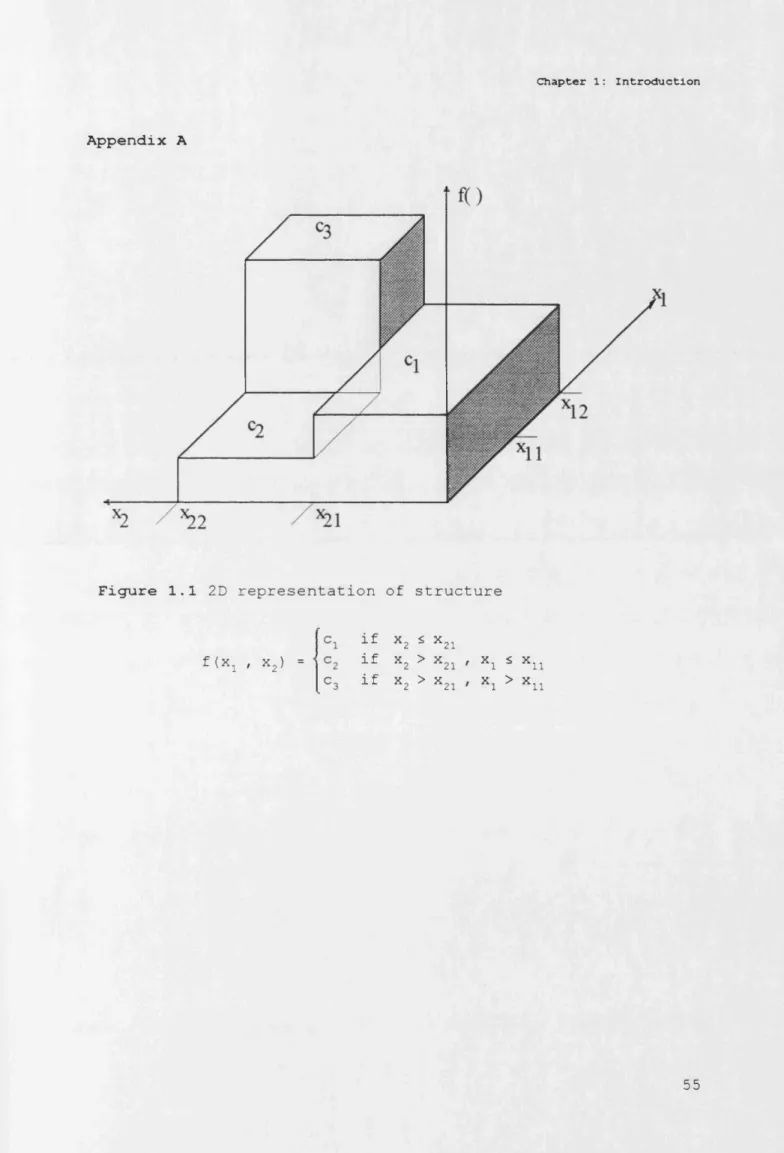
Consider, as an example, the following tree structure defined

on the set C2={[0,xi2], xi26R, i=l,2}

f(xx , x2)

if x2 £ x21 if x2 > x21 if x2 > x21

x i * x n

xi > xii

(1.16)

Figure 1.1 in Appendix A shows a two-dimensional representation

of this three-dimensional surface. If the structure had more

inputs, it would not be possible to draw this graph.

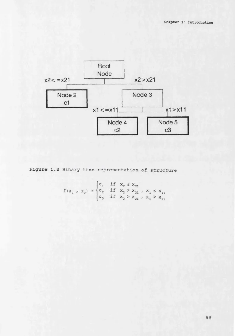
The same structure can be represented by Figure 1.2 in Appendix

A. This figure is a binary tree diagram. Each brand represents

a split of the input space. Each node of the tree represents a

subregion of the space. The root node represents the entire

space. The terminal nodes represent the regions, t, associated

with partition T.

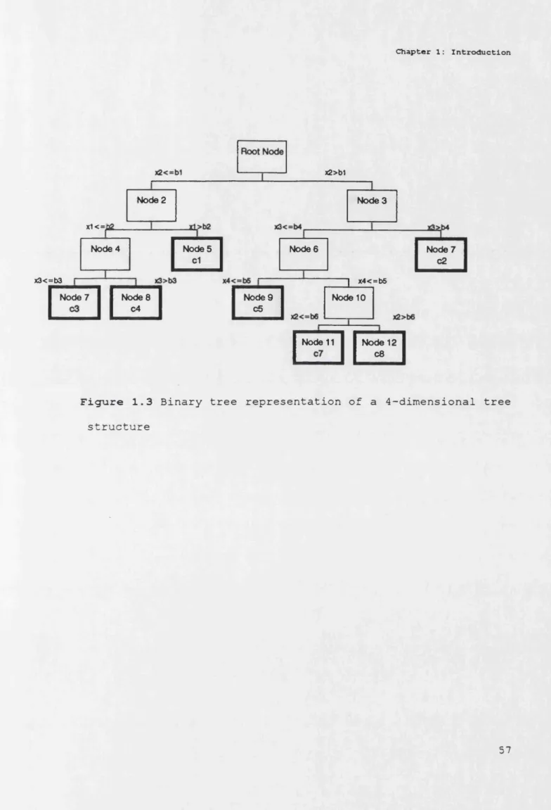
Another example of a tree structured model is shown in Figure

1.3 in Appendix A. The dimension of the input space is four.

Thus, it is impossible to draw something like Figure 1.1.

Nonetheless, all the relevant information that can be obtained

from graphs such as Figure 1.1 can also be obtained from tree

(26)

of edges.

The most important assumption in tree models such as (1.16) is therefore the existence of sudden changes in the flat surfaces.

This is a very bad assumption if the surface changes smoothly.

Another problem is the possibility that the surface does not

change along parallel lines from the axis. Figure 1.4 represents

a structure with these two features. These shortcomings suggest

generalizing (1.15) to propose

General models along this line have been implemented. They

mitigate the rigidity of the activation function by looking at

a very large number of splitting criteria and a large number of

surfaces. The cost comes both in terms of the complexity of the

efficient algorithms and the interpretation of the results.

1.1.5 Universal approximators

In the artificial neural networks literature, the models

reviewed in the previous sections are often interpreted as

approximations of the true model. A universal approximator is

a flexible functional form that can approximate an arbitrary

function to a particular level of accuracy. Neural networks,

projection pursuit and trees all share the functional form

h T(x|x € t) = ft(x, a fc) . _(1.17)

(27)

Chapter 1: Introduction

These models are also universal approximators for the class of

all continuous functions in the sense that any arbitrary

continuous function f (•) admits the representation

oo

f(x) = £ a t • b ( x, y ) (1.19)

t-i

for some set of sequence coefficient values7 {am}“. Therefore,

these nonparametric models have similar spanning properties as,

for example, polynomials.

In spite of this result, it is reasonable to expect that in

small samples selection of the method becomes critical.

1.2 Estimation of regression trees

The original problem of estimating (1.15) is rather trivial if we know the tree structure. Since the constant c which minimizes

E [ (y-c) 2|xet] is E[y|xet], then the least squares estimator, LS,

is the sample average within each terminal node.

If we do not know the structure of the tree, then LS will not

be in general implementable for even not-too-high dimensional

problems. The reason is that LS will be a combinatorial -not an

analytical- problem in this context. In order to minimize (1.3)

one should evaluate all possible structures. This is an enormous

(28)

task. Consider LS on a sample with 50 different cells assuming

that the structure has at most two terminal nodes. The number

of possible models is near 6xl014. This is a very big number. If

we could process every iteration in a millionth of a second, we

would obtain LS only after 17 years of uninterrupted

computations. Given the state of computer technology other

alternatives must be considered.

A second best solution of the problem is recursive partition.

The initial region is divided into two regions according to a

splitting criterion. Then, recursive partition is carried out

on each region. This strategy is implementable because, as

partitioning takes place, the corresponding regions -nodes in

tree terminology- include smaller and smaller subregions of the

original input space. The number of nodes increases at every

step, but each node becomes ever more local. An essential

feature in the procedure is that splitting of each region is

assessed only by studying a limited number of possible splits.

Let us now describe the splitting or tree-growing algorithm.

Assume that we have already several nodes and a tree structure

T and that we want to split node t*, one terminal node in T.

Define d(x) as the tree structure projections from T. The

average residual sum of squares for tree T is

(29)

Chapter 1: Introduction

where N is the number of observations in our estimation sample.

We can also express R(T) explicitly as a function of the

residual sum of squares within each terminal node of the tree.

Then, (1.20) becomes

R(T)

= ^ E E (

Yi

"

^ ( x j ) 2 (1.21)

N teT Xjet

where d ( x±) = (1/Nt) • £ xet y ± .

Recursive partitioning is defined through recursive

optimization. Heuristically, when a variable has a strong

contribution to the true tree structure, a split based on that

variable will likely improve the fit and thus reduce R(T)

greatly. Thus, recursive partitioning can be defined by choosing

the split at each step of the algorithm such that the reduction

in R(T) is maximized. The split chosen at each step of the

algorithm, s*, satisfies

AR(s*,T) = max R (T) -R(T ) , (1 2 2 )

ses

where Ts is any tree obtained by splitting a terminal node, t,

into a left node, tL, and a right node, tR. Since

R(T) - R(TS) = i E ( Yi - d(Xi))

N,I‘et , (1.23)

-

TT

E <

Yi - d U , ) ) 2 - _

E

( Yi - d (xi))2

iN x e t _{i L} JN x e t

(30)

optimal split at each two new terminal nodes from the previous

split.

We can keep splitting the estimation sample until there are no

nodes with elements with different characteristics or the number

of observations reach a lower limit. This lower limit can be

fixed by the researcher according to the problem and is called

the splitting rule. Splitting ends when we obtain the largest

possible tree, T,^. Often, the result will be equivalent to

dividing the sample into all possible cells and computing within

cell averages, a standard nonparametric analysis.

Growing the tree until no further partitioning is possible helps

avoiding having to select a rule to stop splitting. Usually,

however, Tj^ will be too complex in the sense that some terminal

nodes could be aggregated into one terminal node. A more

simplified structure will normally lead to more accurate within

node estimates since the number of observations in each terminal

node grows as aggregation takes place. It is also intuitive to

see that if aggregation goes too far, aggregation bias will

become a serious problem.

In order to aggregate from we can use a clustering algorithm

procedure8. Breiman et alia (1984) propose to compute the

See e.g. Gordon (1993) and Hartigan (1975) for

(31)

Chapter 1: Introduction

error-complexity measure R(Q',T)=R(T)+ojT| for all possible trees

obtained from simplifying the structure by cutting, or pruning,

tree TV^. Here, |T| denotes the number of terminal nodes in T,

that is, the complexity of the tree, and O' is a given parameter.

Note that R(ar, T) is an error-complexity function by which a

model is selected trading variance with complexity.

The tree structured estimate for a given a is the value that

minimizes R(Q7 T) for the set of subtrees of The resulting

tree belongs to a much broader set of trees than the sequence

of all trees obtained in the recursive partition algorithm.

Heuristically, part of the harm done by recursive partition is

reduced. Thus, regression trees are much more powerful pattern

recognition tools than ordinary clustering algorithms.

Optimization of the error-complexity function for a l l possible

values of a leads to an increasing finite sequence of real

values 0 = a 1< a 2< • • • <qq anc* a decreasing finite sequence of

subtrees T1>T2> ...>{root}, such that for any real value

Gk+i) r Tk is the smallest subtree of T,^ minimizing R(o,,T). See

Breiman et alia, (1984, p.289) for a proof of this result.

Implementing cost-complexity minimization for all a is then

possible through a weakest-link algorithm.

an alternative use to clustering algorithms in time series

modelling. See Scott and Symons (1971) and Bryant and Williamson

(32)

Any branch, Tt, spanning from a nonterminal node t of a tree T,

is cut only if

•i E (

yi - d<*i>

>2

+ « s

1

E E <

y± - d(Xl>

>2

+ alTtI»<i.

24

)

N * i « t W t * e T t x ^ t *

so that the first branch to be cut minimizes

E (

yL

- d(x

.))2

- £ E (

yt

- d

(

Xi))2

*iet___ f«Tt »,«t- (1.25)

|Tt| - 1

The initial intractable problem is thus reduced to one of

selecting an optimum-size tree from a decreasing sequence of

subtrees.

At each step of the pruning algorithm R(T) increases so that

R(TX) is the lowest value of the sequence {TX>T2 >. . . >{root}} . For

the learning sample, our estimates d(x) from Tx are therefore

least squares estimates among the sequence. This property is

satisfied in the estimation sample by definition, but it does

not have to do so in an independent sample. Choosing R(TX) as

our fit of the tree structured model may lead to overoptimistic

results for R(*) and the model will be overfitted.

There are three strategies to obtain unbiased estimates of R(*)*

The first one is the use of an independent test sample. This is

most appropriate, due to its simplicity, when the data set has

(33)

Chapter 1: Introduction

entire sample into a learning and a test sample. The tree is

grown and pruned with the learning sample, while unbiased

estimates of R(T) , Rts, can be obtained with the observations of

the test sample and the estimates of the learning sample.

The other two alternatives to obtain unbiased estimates of R(*)

are K-fold cross-validation and the bootstrap method. Since they

will not be implemented in the following chapters, I refer the

reader to Breiman et alia (1984) for an introduction to the

application of these methods in regression trees.

It is possible to compute standard errors for Rts from the test

sample, SE(Rts). Rts may be very flat along the sequence only to

increase at the last, coarser subtrees. When this happens it may

be difficult to justify the least squares subtree and it is

probably better to study several alternatives. Breiman et alia

(1984) suggest the 1 SE rule, which consists of selecting the

simpler tree whose Rts is not larger than the minimum Rts plus

1 standard error. Using these corrections may greatly reduce the

number of terminal nodes of the tree. In the regression trees

literature, sometimes this is referred to as the goal of

obtaining parsimonious models. In a more general context

parsimony and complexity are, however, different concepts. For

example, in a simple linear model with one continuous

independent variable, complexity is infinity, whilst we can

still talk of a simple parsimonious model. In parametric

(34)

reducing the number of projected values for the dependent

variable -complexity-, but also through the estimation of simple

relations between the dependent variable and the independent

variables. In the following, I will nonetheless use the concepts

of parsimony and complexity as interchangeable.

The small sample statistical properties of the estimator just

described are not known. This problem is not trivial because the

technique involves partitions of the input space based on the

learning sample. Thus, the estimates are the results of random

partitions.

Nonetheless it is possible to know something about the behavior

of the recursive estimates as the sample becomes larger and

larger. The fundamental consistency conditions for random

partitions are surprisingly general. All we need is an ever more

dense sample at all n-dimensional balls of the input space in

order to approximate in a q-square sense the nonparametric

surface. If the partition guarantees this, then the estimates

should converge to the true function. Cost-complexity

minimization together with test sample unbiased estimates of

R ( • ) guarantee that such condition is satisfied by regression

tree partitions. The basic results can be found in Breiman et

alia (1984, chapter 12).

A word of caution is nonetheless necessary. For small samples,

(35)

Chapter 1: Introduction

instability in the tree topology so that slight changes in the

learning sample may cause splits to be made on different

variables. In this case, the interpretation of the contribution

of each variable will become problematic.

1.3 Regression trees in economics

Although regression trees has been used in several scientific

fields such as medical diagnosis, automatic identification of

chemical spectra and pollution level predictors in urban areas,

its implementation in economics has been to date rather small.

Nonetheless, we have seen some examples of implementation of the

technique in economics during the 90s. Here I present a brief

summary of three of them.

They highlight in my view its potential applicability to study

economic issues. In the following section I will argue that the

study of wages is a field where this technique can be

interesting to apply.

1.3.1 A classification algorithm

Cotterman and Perachi (1992) describe a method for deciding how

to aggregate a set of elementary U.S. industries. The method is

based on regression trees methodology and it is an alternative

(36)

much broader set of aggregation alternatives.

The fundamental difference with respect to standard regression

trees is that their methodology simplifies the first algorithm,

growing-the-tree, into a simple clustering algorithm. The second

step corresponds to pruning-the-tree. Finally, since they are

only interested in reporting alternative levels of industry

aggregation, they do not implement cross-validation, but present

the differences between their aggregation techniques and the

15-industry level proposed be the U.S. Bureau of the Census.

In order to grow the tree, they propose two measures of

closeness between the elementary industries. First, using data

from the Current Population Survey prepared by the Bureau of the

Census, CPS, and a matching algorithm, it is possible to have

for some individuals two independent codings of the industry of

employment. For some workers, however, these codings do not

coincide. Further, they seem to affect some pairs of industries

more'than others. The authors attribute them to three potential

causes: data collecting errors, errors in the matching algorithm

or, finally, ambiguity in the definition of the elementary

industries. They assume that the last cause is the relevant one

and propose mismatch rates between industry codings as measures

of similarity. The second proposed measure of industry closeness

is the workers' transitions between industries. The measure is

reasonable when individuals move more frequently between similar

(37)

Chapter 1: Introduction

algorithms. Both measures led to different results for the

hierarchical tree. It is interesting that the authors depart

from common practice in clustering when they propose these

measures. The usual procedure is to define closeness through a

distance based on a vector of characteristics. They tried to

overcome the arbitrary step of defining this vector.

Optimal pruning using log-wage data for the years 1971-1982

again from the CPS was carried out. Residual sum of squares were

obtained from regressions of weekly wages on years of schooling,

years of experience and its square. The authors find important

differences in the various aggregation schemes, and conclude9

that since "(...) the outcome of much applied work may hinge on

the aggregates employed", then " (...) procedures for

classification and aggregation are legitimate and important

subjects of inquiry".

1.3.2 Melon prices

Russel Tronstad (1995) applies regression trees to estimate

discounts and premiums due to various characteristics of

wholesale melons. Characteristics considered are melon type,

size, grade, shipping container, week, and year.

Melons are highly perishable products, so that supply of melons

(38)

can be assumed to be perfectly inelastic. After correcting from

season, differences in prices between different types of melons

thus show differences in demands that are due to differences in

the characteristics, not in relative supplies.

The model was estimated with weekly price data from 3 January

1990 through 28 December 1993. Twelve different melon types were

considered. The data source was the L o s A n g e l e s W h o l e s a l e F r u i t

a n d V e g e t a b l e R e p o r t , published by the U.S. Department of

Agriculture.

The results compared favorably to standard parametric regression

in the sense of a higher coefficient of determination. The

author also considers that regression trees performed better

since it allowed for interaction between discrete variables.

Allowing for these interactions on the OLS regression would have

required a very large number of dummy variables. Efficient

estimation would have then demanded the implementation of some

model selection algorithm.

1.3.3 Multiple growth regimes

Durlauf and Johnson (1995) use regression trees to identify

national economies with different laws of growth.

They argue that a cross-section linear regression applied to

(39)

Chapter 1: Introduction

states can produce a negative initial income coefficient. Thus,

a negative sign in this coefficient cannot be taken as evidence

of convergence in income per capita for all countries.

The data source is Summers and Heston (1988) and the World

BankTs W o r l d T a b l e s and W o r l d D e v e l o p m e n t R e p o r t . The authors

initially carry out ad hoc splits of the countries into two,

three and four groups based on their initial per capita output

and literacy rates. They then test for the existence of a common

growth path for these groups. They reject the null hypothesis

against the alternative of multiple regimes in a human capital

specification and in an augmented version that tries to

incorporate social and political factors. In both cases, they

reject the hypothesis of a single growth regime against the

hypothesis of several regimes.

Regression trees allows for endogenously finding the number and

specification of growth regimes. The splitting criteria in the

tree are based on initial literacy rates and income per capita.

This is consistent with the multiple regime framework since if

economies are concentrated around several steady states, then

their initial values for these variables will cluster for each

group. Within nodes sum of squares are computed from the

residuals of the growth equations.

The algorithm partitions the world economy into four groups and

(40)

economies have access to different aggregate technologies.

In the following section I will consider the use of regression

trees in the study of the wage structure. I will present

empirical results that highlight the strong context-sensitivity

feature that wages present in the U.S.. I will then give an

outline of the rest of this volume and will end with a

description of the data and programming to be used in the

following empirical applications.

1.4 Nonparametrie Wage- Structures

1.4.1 Wage structures

The concept of the wage structure is fundamental in the

empirical analysis of the characteristics of the wage

distribution. It refers to the vector of prices set for various

labor market skills and the rents received for employment in

particular sectors of the economy.

The labor market is seen as a complex structure that consists

of interrelated local markets with different market equilibrium

wages. A description of this structure and its evolution is of

clear interest to study problems as varied as the effects of

technological change, the sources of wage inequality, and

(41)

Chapter 1: Introduction

We can start by simply assuming that the logarithm of the

market-clearing wage for any worker, wif depends on observed and

unobserved characteristics that position the worker in a segment

of the labor market.

It is customary to assume a linear relation between the observed

and unobserved effects, where the unobserved effect term will

have zero expected value and small variance a2. The general

specification for the econometric model in this literature is

then simply

w. = f(x.) + v. . (1.26)

The simplest and commonest specification for (1.26) is a

polynomial parametric relation between the explanatory

variables. For example, a squared term for experience on top of

a linear model is usually included since the publication of the

seminal work of Mincer (1974) 10.

The linear parametric approach implies that each variable’s

additional contribution to wages is constant or follows a

10 It is customary to refer to a wage equation that is

linear on the education level, experience, and experience2 as a

Mincer equation. The conection between human capital models and

this simple specification was one of the main contributions of

Mincer. This is nowadays sometimes recognized by referring to

(42)

be solved by adding just a few quadratic terms in the right-hand

side of the equation? My intuition is that it cannot. By

postulating a rigid structure, the researcher may distort the

information available in the data set so that the results will

not be useful.

In the next section, I will review the empirical evidence on

context sensitivity in the U.S. wage structure.

1.4.2 A survey on context sensitivity in the U.S. wage structure

There is a remarkable consensus in the economic literature on

the recent general trends of relative wages. It seems that the

fundamental dynamic features of wages are sufficiently well

described along just three or four dimensions.

First, there was a general trend of wage dispersion and a slow

down of growth in real wages during the eighties. Second, there

have been increases in the wage differentials between workers

with college and high school education for all demographic

groups defined by gender and age. Experience differentials have

continued a long-term increasing trend. On the other hand,

gender differentials narrowed further while race differentials

reported that the parameters of these terms were not

significantly different from zero when wages instead of earnings

(43)

Chapter 1: Introduction

remained stable in the last twenty years. Industry differentials

have also remained stable.

Compared with the trends observed in the sixties and seventies,

the growing inequality in the eighties was not a unique

phenomenon. Wage dispersion within groups and increases in

experience differentials were not new trends. However, the

reductions in the College premium during the 1970’s and the

narrowing of the race differentials before 1975 did not occur

later13.

On top of these general stylized facts we can find many reported

local cases of context sensitivity or nonhomogeneity in wage

differentials. Probably the best known of these is the different

behavior of the experience differential between high school and

college graduates. It seems that the combination of college

attendance and job experience was an unbeatable one during the

13 See, for example, Levy and Murname (1992) and Bus chins ki

(1994). Allen (1995) analyzes changes in the wage structure

across manufacturing over the years 1890-1990. He concludes that

interindustry wage differentials were highly stable over the

entire period for production workers. Interindustry wage

(44)

eighties14. Welch (1979) argued that college graduates are more

imperfect substitutes for more experienced graduates than is the

case for workers with less education.

Similar asymmetries can be found along other demographic

dimensions. Let us consider the interaction between education

and race. While the college-going rate for 18-24 year old,

white, high-school graduates increased from 31.2% to 38.1%

between 1979 and 1987, the college going rate for black high

school graduates in this age group fell from 29.5% to 28.1%,

suggesting that the college premium has a race story inside15.

The race differential for women almost disappeared in the 1970s,

while it remained stable for male16. Thus, either the wage

structure is becoming nonhomogeneous with respect to the race

differential, or it never was.

Some authors have studied the relationships between sector of

employment and race. Greene and Rogers (1994), for example, find

important differences between the private and public sectors

with respect to earnings of college-educated black and white

14 See, amongst others, Bound and Johnson (1992), Katz and

Murphy (1992), and Murphy and Welch (1992).

15 See Levy and Murnane (1992) and also Ashraf (1995).

16 See, for example, Murphy and Welch (1992) and Blau and

(45)

Chapter 1: Introduction

professionals.

Bound and Holzer (1993) estimate the effects of industrial

shifts in the 1970s on the wages and employment of black and

white males and find that while the magnitudes of these effects

are fairly small for many groups, they can account for about 40-

5 0 percent of the employment decline for less-educated young

blacks.

Firm and industry effects have also been compared on several

occasions. Davis and Haltiwanger (1991) find that steady growth

in wage differentials among plants in the manufacturing sector

between 1975 and 1986 accounts for half of the growth in wage

dispersion within this sector17.

Bound and Johnson (1992) find that when 45 instead of 17

industries were used for "all men” and "all women" groups, most

17 It is unclear whether this pattern extends to other

industries, particularly after considering that international

competition may have increased the pressure on firms to choose

between quality improvements or cost reductions in the labor

force. Levy and Murnane (1992) argue that the eighties may just

have been a period of adjustment for the manufacturing sector

that will end when those firms which chose the losing strategy

(46)

of the industry effects were picked up by the dummy variables

for 17 industries. The interesting exceptions were non-college

men during the 1980 fs, for whom the use of detailed industry

dummies increased the total industry wage effects by up to one-

half .

Blackburn (1990) shows that approximately 15 percent of the

increase in within-group variation for men stems from the

movement of workers from goods producing industries to services.

Other variables of potential interest have also been studied and

their interactions locally analyzed. A few examples follow.

There is no clear consensus on regional variations and their

effects on the wage structure. Eberts and Schweitzer (1994) find

that the trend in regional variation can be traced to declining

differences in labor market valuations of worker attributes

rather than to shifts in the regional composition of the

workforce. See also Gyimah and Fichtenbaum (1994) for an

investigation on the regional differences in labor market gender

and race discrimination. Larger differences do not imply larger

discrimination.

Immigrants with lower initial wages were assimilated in the U.S.

market faster than those with higher initial wages (LaLonde and

(47)

Chapter 1: Introduction

Social status has also been considered: Among males, growth in

the proportion of males in the labor force who are unmarried has

affected the married status differential18.

Finally, Adamson (1993) study differences in union affiliation

relative wages across gender and race and finds that the female

union effect declined over the 1970-1982 period whilst the size

of the male union effect remained stable.

The list of cases is not at all exhaustive. The examples

nevertheless transmit the message that local analysis unveils

context sensitivity. This is done by focusing on the

interactions of at most three variables. Note that in order to

observe context sensitivity using parametric techniques we must

include at least quadratic effects in the set of explanatory

variables or, more generally, estimate different wage equations

in different segments of the labor market. This, in effect,

eliminates the possibility of a global context-sensitive

parametric approach.

From the extensive literature on wage premiums we must conclude

that any global analysis of wages may suffer from aggregation

bias and that even local studies should take account of

nonhomogeneous features in the structure.

(48)

It seems therefore desirable to keep the empirical analysis to

the highest level of flexibility. A nonparametric approach over

all possible points of the input space cannot be used for

practical reasons. A simple example will fix ideas. Bound and

Johnson (1992) did not try a very detailed specification of the

input space. They took three periods (1973-1974, 1979, and 1988)

and for each of them the population was divided into 32

subsamples -according to education, potential labor market

experience and gender- on which wage regressions were carried

out with dummies for the following characteristics: Educational

attainment, nonwhite, part-time employment, residence in an

SMS A, four major regions and employment in 17 major industries.

The most complex nonparametric surface would involve 15,000

different labor groups. In order to have at least 50

observations for each type of worker, the research can only be

carried out with samples of at least 750,000 observations.

Thus, it seems that ad hoc searches for the best functional

local parametric specification is the only available strategy.

It is not. Parsimonious nonparametric econometric models such

as regression trees allow for simple nonparametric structures

in the sense of a low number of different expected equilibrium

wages19. They thus provide a very useful tool in the study of

local segments of the labor market.

19 This is the result when the splitting rule constraint is

(49)

Chapter 1: Introduction

1.5 Outline of the thesis

1.5.1 Outline of the thesis

The fundamental econometric problem that model (2.1) may have

is related to the statistical relation between the observed

variables and a subset of the unobserved variables. The general

idea is that if economic agents take decisions based on an

opportunity set not observable to the researcher, and if

opportunities vary across agents, then observable data will be

censored and the error term may not be independent of one of the

regressors.

In the context of measuring the returns to education, this self

selection/omitted variables problem would imply that OLS

estimates of the education coefficient may be upward biased.

Intuitively, individuals with higher ability, an unobservable

variable, will normally choose higher levels of schooling

because they can benefit most from it (e.g. Griliches (1977)).

The interpretation of the importance of the education variable

in the estimated tree will also present the same problem.

In the context of gender differentials, participation decisions

in the labor market censors especially female data. Again, LS

estimates will be biased if the decision to participate is

(50)

as education. The same problems affect again the interpretation

of the gender estimate in regression trees.

It is possible to define regression trees so that these problems

can be addressed. The main idea is to use standard parametric

regression techniques designed to cope with these problems at

each node instead of simple within node averages in order to

estimate the impurity at each node. This is, no doubt, a very

interesting direction to enlarge this study.

In the rest of the thesis, I will present, however, the results

of applying the simplest regression trees algorithms to samples

of populations for whom, I will argue, the econometric problems

just mentioned are minimized.

Three applications of regression trees on the study of the wage

structure are implemented in the following three chapters of

this dissertation:

a.- I will first estimate experience-wage profiles for

white male full-time employed workers.

b.- Secondly, I will decompose average wage differentials

of different groups using nonparametric structures estimated by

regression trees.

(51)

Chapter 1: Introduction

nonparametric wage structures estimated by regression trees.

Obviously, the choice of the subjects probably reflects mostly

the interests of the author and I would not like to suggest that

these fields are the most promising for the application of

nonparametric multivariate techniques to the study of wage

structures.

Before turning to the results of the empirical applications, I

would like to comment on the data set and the programming

language used.

1.5.2 Data and programming

In the following chapters I will use the outgoing rotation

groups of the Current Population Survey (CPS). The Current

Population Survey is a monthly survey of now about 60,000

households prepared by the Bureau of Labor Statistics, BLS. An

adult (the reference person) at each household is asked to

report on the activities of all other persons in the household.

There is a record in the file for each adult person. The

universe is the adult noninstitutional population.

Each household entering the CPS is administered four monthly

interviews, then ignored for eight months, then interviewed

again for four more months. If the occupants of a dwelling unit

(52)

unit are interviewed. Since 197 9 only households in months

fourth and eighth have been asked their usual weekly

earnings/usual weekly hours of work. These are the outgoing

rotation groups, and each year the BLS gathers all these

interviews together into a single Merged Outgoing Rotation

Group. A consequence of this construction is that an individual

appears only once in any file year, but may reappear in the

following year. The National Bureau of Economic Research, NBER,

has prepared a CD-ROM with extracts of the files.

These data have, however, some limitations as a data set for

studying the evolution of wages across different groups20. I will

comment on four problems that may distort results.

First, the definition of income does not include fringe

benefits, which have constituted a rising proportion of income

compensation. Levy and Murnane (1992) argue that after adjusting

for fringe benefits the difference between the rates of growth

of real wages for the sixties and eighties diminishes, but the

eighties value is still well below the pre-1973 period.

Second, to preserve confidentiality in the upper tail of the

income distribution, the statistics reported are top-coded at

$50,000 from 1968-1981, $75,000 from 1982 to 1984 and $99,000

20 For a more detailed discussion, see Levy and Murnane

(53)

Chapter 1: Introduction

from 1985. This problem can actually be lessened by avoiding all

together the tails of the distribution although more

sophisticated procedures have been proposed21.

The fact that the CPS lacks information on firm specific

activities can be important if workers have heterogeneous

characteristics and production potential across firms.

Finally, the CPS data may overstate the rate of growth during

the 198 0 ’s in the proportion of new labor market entrants who

were college educated and underestimate the earnings of workers

who completed a normal high school programme. Bishop (1991)

finds an unprecedented mismatch in the 1980's between the CPS

data on new entrants who had accomplished college education and

the number of degrees awarded in the U.S.. With respect to high

school graduates, before 1988 the CPS treated both holders of

the General Educational Development exam and traditional high

school graduates as having completed 12 years of schooling.

However, Cameron and Heckman (1991) find, with data from the

National Longitudinal Study of Youth data set, that the first

group earnings patterns are indistinguishable from high school

dropouts.

21 Truncation corrections for top coding normally assume a

gamma distribution for the upper tail of the yearly income

(54)

I implemented regression trees algorithms on large data sets of

wages. The computations were carried out using the author's

procedures programmed in GAUSS for regression trees on ordered

variables. An interesting feature of the chosen programming

language was the possibility of using a simple matrix

programming language together with large data sets. In

particular, the procedures were able to process sets with more

than 60,000 observations with speed in a personal computer and

limited memory. Available commercial software would not do the

(55)

Chapter 1: Introduction

Appendix A

Figure 1.1 2D representation of structure

f(xx , x 2) =

if x2 s x21 i f X2 > X21

if x2 > x21

X 1 s x u

X 1 > x u <

Use of regression trees in the study of nonparametric wage structures