Improving Geocoding Rates in Preparation for Crime Data Analysis

University of East London Institutional Repository: http://roar.uel.ac.uk

This paper is made available online in accordance with publisher policies. Please scroll down to view the document itself. Please refer to the repository record for this item and our policy information available from the repository home page for further information.

To see the final version of this paper please visit the publisher’s website. Access to the published version may require a subscription.

Author(s):Brimicombe, Allan. J., Brimicombe, Lily C., Li, Yang.

Article Title:Improving Geocoding Rates in Preparation for Crime Data Analysis

Year of publication:2007

Citation:Brimicombe, A.J., Brimicombe, L.C., Li, Y. (2007) ‘Improving Geocoding Rates in Preparation for Crime Data Analysis’International Journal of Police Science & Management 9 (1) 80-92

Link to published version:

http://search.ebscohost.com/login.aspx?direct=true&db=a9h&AN=24405752&site=eh ost-live

DOI:(not stated)

Publisher statement:

http://www.vathek.com/permissions.php

Improving Geocoding Rates in Preparation for Crime Data Analysis

Allan J. Brimicombe1

Centre for Geo-Information Studies, University of East London, University Way, London E16 2RD, UK

Lily C. Brimicombe

Terra Cognita, Wrights Green, Bishop’s Stortford, Hertfordshire, CM22 7RJ, UK

Yang Li

Centre for Geo-Information Studies, University of East London, University Way, London E16 2RD, UK

Abstract

Problem-oriented policing requires quality analyses of patterns and trends in

crime incidences. Included within this is the identification of geographical clusters or hot

spots. Crime incident records must first geocoded, that is, address-matched so as to

have X,Y grid co-ordinates attached to each record. The address fields typically have

omissions and inaccuracies whilst a good proportion of crimes occur at non-address

locations. This results in the geocoding having an unacceptably low hit rate. We present

and test an improved approach to geocoding of crime records that raises the hit rate by

an additional 65% to an overall rate of 91%. Kernel density surfaces show that these

additional geocoded records have distinct spatial patterning which, furthermore, indicate

1 _{Corresponding author: Tel: +44 (0)20 8223 2352 Fax: +44 (0)20 223 2918}

that without the improved hit rate, hot spots of crime also tend to be hot spots of missing

data.

Keywords: spatial databases and GIS, clustering, data cleaning, geocoding, crime

mapping.

1. Introduction

During the 1980s and 1990s policing in North America and Europe progressively

shifted its focus from a reactive incident-driven approach to a pro-active problem-solving

approach. Problem-orientated policing [1, 2, 3] is an underlying philosophy which

suggests that policing is not just about enforcement of the law but should be more about

solving underlying problems within the community – not just catching criminals but

working in partnership with other agencies towards crime prevention. Underlying most

approaches to problem-oriented policing and crime prevention is the understanding that

crimes tend to form patterns [4]. These patterns are the discernible manifestation that a

repetitive process is at work which, once understood, can be modified or stopped

through an appropriate set of interventions that may be legal, social and/or situational.

The patterning of crime occurs in one or more key dimensions: spatially, temporally or in

the attributes of the modus operandi (MO). The patterns of most interest would either

form a clustering or exhibit a degree of regularity. Both have an element of predictability.

Geographical Information Systems (GIS) have been used since the early 1990s to assist

in identifying geographical clusters of crime, commonly known as hot spots [5, 6, 7].

Crimes are taken as discrete point events recorded as occurring in a specific

include date and time, details of victim(s), MO and description of offender(s). These will

be recorded against specific fields (often as codes) in a database by the reporting officer

either from notes made at the scene of a crime by him/herself and colleagues, as

reported at a police station or from statements made over the phone. There are also

free-text fields used to incorporate longer descriptions of an event. By way of example,

the crime recording system for one metropolitan police force in the UK is organized into

78 tables to record over 700 possible variables of a crime using a unique crime number

to join the tables. The volume of crime for this same metropolitan area, requires the

recording of just over one million crimes each year – an average of 2 every minute. Even

with a commitment for due diligence and attention to detail on the behalf of police

officers, the volume of crime in relation to the size of the police force means that

omissions and inaccuracies are inevitable. Data quality is thus a recurrent issue for

crime data analysts [8, 9] and has important repercussions in drawing tactical and

operational conclusions from analyses. One difficulty faced by UK police forces is in

consistently and accurately locating crimes geographically. Unlike in the US, for

example, where street patterns are predominantly rectilinear and their naming may form

some numerical or lettered progression, UK urban street patterns tend to be sinuous,

dense and complex – accurately recording all elements of an address often necessitates

asking a local resident. Address fields in databases are designed around identifying an

individual property leaving non-addressed locations (e.g. a recreational park, road

junction, bus station) to be recorded/described in free-text fields. When it comes to

mapping crimes as point events, it can easily be the case for some crime types (such as

street crime) that considerably less than 50% of the records can be cartographically

obvious consequences for the reliability of any further analysis and decision-making, are

by no means confined to the UK [5].

In this paper we present an improved and tested approach to increasing the

mapping rate of crime data so as to make crime analyses meaningful. This approach

incorporates data cleaning, text mining, specially prepared gazetteers and novel

reconfiguration of data sets. We begin by briefly reviewing the key methods for

identifying geographical patterns in mapped crime data and hence the significance of

data quality. We then discuss the general means by which logged location records of

crime incidences are batch converted to map co-ordinates (geocoding) and the

problems that arise. We then present details of our improved methodology for

geocoding. Finally we provide evidence of the comparative performance of the

methodology on 90,904 crime records and discuss the implications of the results.

2. Approaches to hot spot detection in crime data

At the heart of problem-orientated policing is the analysis of crime data within the

framework of the problem analysis triangle (PAT) [3, 10] which focuses on the three key

facets of any incident: the incident location, the victim and the offender. Not only does

incident location furnish important environmental variables that may be conducive to or

regularly associated with certain types of crime [11], but the spatial relationships

between incidences and the geographical clustering of crime add understanding of

overall trends and risks of re-victimization [7, 12]. High crime areas are primarily so

because they are areas of high repeat offending and high repeat victimization [13, 14].

Thus existing crime patterns are a usable predictor of future victimization [15]. GIS are

use in the detection of hot spots has been extensively discussed in the literature [5, 6,

12, 16, 17, 18, 19, 20]. Yet, there is no standard definition of a hot spot. The most

commonly understood meaning within police forces focuses on crime counts: an

elevated share of crime in a localized area. The process begins with geocoding, that is,

by matching the address or some other location identifier of an incident with grid

co-ordinates stored in a geographical base file (GBF). The distribution of crimes can thus

be displayed as points against a map backdrop and analyzed alongside their own and

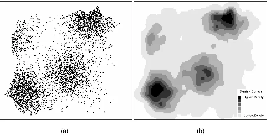
other attributes. Early electronic displays of ‘pin maps’ (such as Figure 1(a)) allowed

subjective judgments of pattern and identification of clusters, but lacked consistency

from one individual to another. Experiments have shown that considerable variation can

arise in the visual perception of clusters in a distribution of point events [21]. Hence the

need for more objective approaches.

A widely used approach to more objective identification of clusters is point density

estimation with functionality available, for example, in CrimeStat®, Spatial Analyst

extension to ArcView® and Hotspot Detective® for MapInfo®. This is an interpolation

that transforms the point events into a gridded continuous surface of density estimates

(incidences per unit area) which is then colored or gray-scaled so that the peaks in the

surface (the hot spots) are easily visualized. The algorithm of choice is kernel density

estimation [22. 23, 24] which uses a Gaussian function across a pre-determined

bandwidth (radius) to provide a smooth estimate of point density that is quick to

calculate (see Figure 1(b)). Although this approach to hot spot detection has been

criticized for its subjectivity in parameter estimation [6, 20], it remains a popular, highly

visual approach that forms an important ‘first sieve’ in focusing attention on high crime

[Figure 1 about here]

It should be clear from the above, that the process of geocoding is a critical step

in achieving quality analyses of geographical pattern and trend within the framework of

the PAT. The ideal would be for 100% of records to be geocoded, but in practice this is

rarely achieved. Few police forces publish their geocoding rates. Quoted figure for the

US [25] suggest a range from 41% to 99.7%. Our experience of UK geocoding rates

prior to the implementation of the methodology presented here would suggest that high

geocoding rates were only achieved after considerable manual plotting of records by

analysts.

3. Issues in geocoding

Geocoding is the process of attaching a mappable spatial identifier to database records.

A mappable spatial identifier is often in the form of X,Y grid co-ordinates (two fields) but

could be a single field containing a numeric or alpha-numeric identifier corresponding to

the primary key in a GIS layer. The fields used in a database for geocoding would be

those corresponding to either a complete address or the generalized elements of an

address (postcode, district). For crime mapping it is desirable to have the highest

resolution and therefore the objective of geocoding is to attach the X,Y grid co-ordinates

of an individual property on the basis of it’s full address. The UK mapping authority, the

Ordnance Survey, produces a GBF for this purpose called Address-Point® which

includes all 27 million addressable properties in the UK and conforms with the Post

Office Address File (PAF) which lists all delivery addresses to British Standard BS7666.

The immediate problem lies with the accuracy with which addresses are recorded

and entered into a crime records system [5, 11, 25, 26]. Entries may not necessarily

conform in structure to BS7666, may contain typographical errors, a range of

abbreviations, omissions or may even be based on inaccurate or purposely misleading

information provided by members of the public. Furthermore, postcodes in the UK are by

no means permanent. They are a device of the Royal Mail (post office) and, having no

statutory basis in law, can and are changed with little or no consultation in order to

optimize mail delivery in response to local changes in the number of delivery points.

Residents often continue to use their former postcode long after it has been changed. A

further issue is that not all places where crimes happen have a BS7666 address.

Examples would be on a railway line, in a public open space or on a bridge. Road

junctions provide address ambiguity as there may be up to four corner properties.

Non-addressable locations and road junctions are usually recorded in a free-text field with the

address fields left blank. Railway stations and other prominent landmarks such as public

buildings are often entered by name with no further address elements.

A number of commercial software products, such as Matchcode® and QAS®,

have been developed to solve many of the common problems associated with

address-cleaning, address-matching and geocoding. These use methods of standardization and

parsing [27] to correct common errors and abbreviations so as to achieve a match with

the PAF and/or Address-Point® and thus attach the grid co-ordinates to a crime record.

In a batch process an unambiguous match to an individual property needs to be

achieved if grid co-ordinates from Address-Point® are to be attached. Whilst in

interactive mode ambiguities may be resolved by an operator in order to increase the

processing thousands of records a month. There are also the non-addressable crime

records which these commercial address-matching products are not designed to solve.

In a test reported below, batch processing using commercial software would typically

geocode only half the records. Whilst analysts may be satisfied to take whatever is

geocoded as a ‘representative sample’, there have been no reported studies of what is

not geocoded so as to establish the extent to which the hit rate might be spatially biased.

Clearly a more sophisticated approach is required.

4. An improved approach to geocoding crime data

A new geocoding toolkit has been developed and tested in order to improve the

hit rate. The toolkit has been created as VBA macros, prototyped in Microsoft® Excel

and ported to Microsoft® Access. Our purpose has not been to replace commercial

address-matching software but to enhance the outcome of the geocoding process by

building additional steps and tools around commercial software. The general strategy

has been to move from the specific to the general, from establishing as accurately as

possible the individual address or road junction, to a small area in the vicinity of the

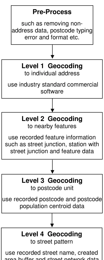
address (postcode) to a section road within a more approximate area. This has resulted

in a five-stage process as shown in Figure 2.

[Figure 2 about here]

The first stage is a pre-process function to clean common errors arising in the

address fields. Whilst some of these may be automatically taken care of by commercial

address-matching software (e.g. Rd changed to Road), a catalogue of minor errors (e.g.

letter ‘O’ mistakenly used instead of number ‘0’ in postcode elements reserved for

process. Also, each address field is checked for consistency and if necessary

inappropriately placed entries are moved to the correct field, any padding is removed

and non-address entries (e.g. ‘car park’ or name of railway station) moved out of

address fields and into new fields for later processing. The effect of this process is to

increase the geocoding hit rate by the commercial software by up to 5%. It also prepares

some of the data fields for subsequent stages.

In the second stage the data are passed through commercial address-matching

software and where an individual property level match is achieved; then grid

co-ordinates are attached by the commercial software from Address-Point®.In the process,

all postcodes are cleaned where possible either from the full address or from a partial

address (road name and district) where there is no ambiguity as to which postcode is

correct. All addresses successfully geocoded at this stage are given the validation code

‘L1’.

In the third stage, the process focuses on non-address locations. The majority of

these are road junctions and can be found in the free-text field describing the venue of

the incident. Other non-address locations would include railway stations, bus stations

and prominent landmarks. The junctions are text mined by searching for keywords.

These include J/W J,W JCT JTN JCTN WITH and other variants. Two road names then

need to be mined out of that free-text field and recorded in separate new fields. In order

to achieve this a pattern recognition exercise was run on a street gazetteer in order to

determine key association rules and ordering. Thus it is theoretically possible to have

Acacia Road, Acacia Hill, Acacia Hill Road and Acacia Hill Road East together with Rd

and Rd. abbreviations for Road and/or E and E. abbreviations for East. A hierarchical

root name e.g. Acacia) and their possible abbreviations. Cardinal directions (North,

South, East , West) are first identified and if found the search continues with the word to

the left. Then finalizations (other than cardinals) such as Road, Street, Avenue,

Approach, Broadway and Drive are searched. When found there is a search for possible

intermediates such as Hill, Dale, Spring and Wood. Finally the root name element is

captured. This process results in two new fields giving two road names that form the

junction. In order to geocode a junction, a lookup database of all junctions and their grid

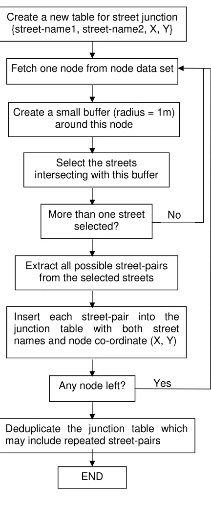
co-ordinates is required. This did not exist. In order to create one, the Ordnance Survey

road center line product OSCAR® was reconfigured using a MapBasic® macro in

MapInfo®. The method is given in Figure 3. The OSCAR® product provides two layers:

a road sections (links) layer and a nodes layer for junctions. Road names are attached

to links, not to nodes. So the reconfiguration process is to intersect nodes with links,

extract the names, organise into pairs of roads coming into junctions, attach grid

co-ordinates and deduplicate the final table. This was then matched with postcodes and

districts and indexed. For the specific metropolitan area for which the toolkit was

created, this new junction database contains 107,355 junction records. Gazetteers of

other non-address locations were also created to facilitate their geocoding. Non-address

locations geocoded in this stage are given the validation code ‘L2’.

[Figure 3 about here]

In the fourth stage, all remaining records with a valid unit postcode are geocoded

at the postcode level. Postcodes in the UK are defined by delivery points, not by a

bounded geographical area. There are on average 15 delivery points per unit postcode

but this number is extremely variable across the UK. For the metropolitan area in this

(approximately 2 acres). The Ordnance Survey product Code-Point® provides

population-weighted centroid co-ordinates for each unit postcode. This has been

produced from Address-Point® records. A simple database join on unit postcode allows

geocoding to take place. Records geocoded in this stage are given the validation code

‘L3’.

The final stage of the toolkit attempts to geocode all remaining records according

to road name. The problem here is that some roads are very long and some road

names, such as High Street, are repeated in different districts. The search needs to be

limited in some way. At the Call and Dispatch centre (CAD), a 250m grid code, the

CADref, is added to an incident record in order to give its approximate location. CADref

can be unreliable but if buffered and intersected with named roads a candidate section

of road could form the basis for geocoding. Again, OSCAR® was reconfigured using

MapBasic® into a file which contained the digitized intermediate points along all links

against road name (procedure in Figure 4). These were then matched with CADref so all

the digitized points of a road falling within a CADref could be identified. The final index

file contains 543,023 records. If a match for road name and buffered CADref (by one half

grid cell on all sides) is achieved then a digitized point for the relevant section of road is

chosen at random and used to geocode the crime incident. This is the least accurate

level of geocoding and records are given the validation code ‘L4’. Nevertheless, the

geocoded crime incident falls on the road specified in the crime record and in the

approximate area of the CADref provided.

5. Results

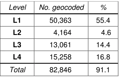
The improved approach embodied within the toolkit was tested by batch

processing one month’s crime records for a large (157 sq. km; 61 sq. mile) metropolitan

area in the UK. This amounted to 90,904 crime records. Table 1 summarizes the hit rate

for each level, with an overall hit rate of 91.1%. The commercial address-matching

software, even after the enhancements of the pre-processing stage, only achieves a

55.4% hit rate (L1). Between L2 (junctions) and L3 (postcodes) another 20% is added.

Surprising is the 16.8% that would then have been left un-geocoded if it were not for the

combination of road name and CADref (L4). The improved methodology has taken the

geocoding hit rate from a position that is clearly unacceptable [25] to one which can be

taken as a sound basis for crime analysis.

[Table 1 about here]

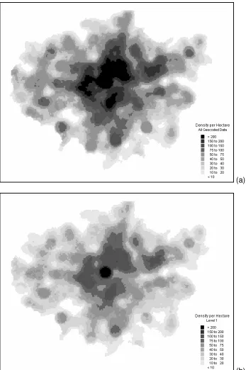
In order to visualize and explore the spatial dimension of Table 1, a series of

kernel density surfaces has been produced using a public domain code for MapInfo®

[28]. In order to be consistent, Figures 5 through 7 have all been constructed using a

500m bandwidth across a 250m grid surface. However, the gray scale legend is different

for Figure 5 as compared with Figures 6 and 7 because of changes in the range of

densities present. Figure 5(a) shows the density surface for all the successfully

geocoded records (L1 to L4). This is the best picture we are going to achieve from a

batch process though some 9% of data is still missing. It shows a concentration of crime

(hot spot) over a wide area of the city center and in the inner city residential areas with

other more or less well-defined hot spots in a number of suburban districts. Figure 5(b)

shows L1 geocoded records. Overall it looks similar to Figure 5(a) but at much lower

crime in Figure 5(b) might be concluded as being much less severe in the absence of

Figure 5(a) with the suburban hotspots appearing much milder than otherwise would be

the case.

[Figure 5 about here]

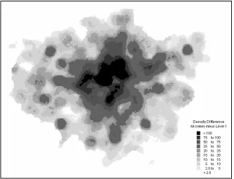
Figure 6 is Figure 5(a) minus Figure5(b). Note the difference in scale of the gray

shading. The feature that is striking is that overall, the pattern presented is similar to

Figure 5(a), suggesting in fact that hot spots of crime are also hot spots of un-geocoded

records. This would seem intuitive if one considers that the intensity of law enforcement

activity within hot spots and the pressures on the police officers detracts from their ability

to carefully and fully record the location of incidences.

[Figure 6 about here]

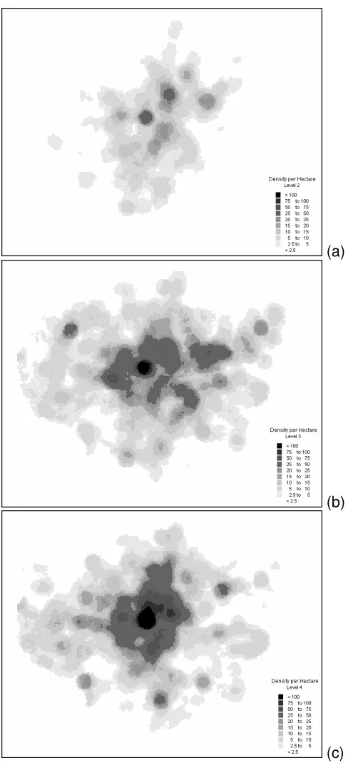
Figure 7 shows density surfaces for L2, L3 and L4 geocoded records. Overall

they show a concentration of poorly addressed records and non-address records that

have been resolved around the inner city. On the one hand the older heart of the city

have the most complex road patterns. Commercial buildings here have a tendency not

to display a number and often company names are recorded instead. This is also the

area with the greatest on-street movement of people (day and night) and concentration

of parked cars and hence a higher propensity for on-street crime compared with other

areas of the city. Figure 7(a) would suggest a distinct spatial bias in L2 (predominantly

road junctions) on a north-south axis across the city center, though the reason for this is

not clear. L3 geocoded records in Figure7(b) shows a tendency to pick out some of the

suburban hot spots, whilst L4 geocoded records in Figure 7(c) picks out others. This

may reflect differing local practices within individual districts in the attention given to

[Figure 7 about here]

6. Conclusions

An improved approach to geocoding of crime data in preparation for crime data

analysis has been implemented and tested. The performance of commercially available

software on their own are not adequate given the particular issues and complexities of

crime records systems. By improving the hit rate through additional processing, a further

65% of crime records can be geocoded as point events to obtain an overall geocoding

hit rate of 91%. This better assures the quality of analyses that may be carried out on

the data. As has been demonstrated, hot spots of crime are also hot spots of

un-geocoded records. The various levels of geocoding, resulting from the new toolkit, each

shows their own strong spatial patterning. This would suggest that if L1 data were to

References

[1] H. Goldstein, “Improving policing: a problem-orientated approach”, Crime &

Delinquency , April 1979, pp. 236-258.

[2] H. Goldstein, Problem-Orientated Policing, McGraw-Hill, New York, 1990.

[3] A. Leigh, T. Read, and N. Tilley, Problem-Orientated Policing: Brit Pop, Home

Office, London, 1996.

[4] P. Brantingham, and P. Brantingham, Patterns in Crime, Macmillan, New York,

1984.

[5] K. Harries, Mapping Crime: Principle and Practice, US Department of Justice,

Washington DC, 1999.

[6] S. McLafferty, D. Williamson, and P.G. Maguire, “Identifying crime hot spots using

kernel smoothing”, Analyzing Crime Patterns: Frontiers of Practice V. Goldsmith, et

al., eds., Sage, Thousand Oaks, CA, 2000, pp. 77-85

[7] P.B. Ainsworth, Offender Profiling and Crime Mapping, Willan, Cullopton, 2001.

[8] P. Ekblom, Getting the Best out of Crime Analysis, Home Office, London, 1988.

[9] T. Read, and D. Oldfield, Local Crime Analysis, Home Office, London, 1995.

[10] Audit Commission, Safety in Numbers, The Audit Commission, London, 1999.

[11] R. Boba, Introductory Guide to Crime Analysis and Mapping, US Department of

Justice, Washington DC, 2001.

[12] G.C. Oatley, and B.W. Ewart, “Crimes analysis software: ‘pin maps’, clustering and

Bayes net prediction”, Expert Systems and Applications 25, 2003, pp. 569-588.

[13] A.Trickett, D.K. Osborne, J. Seymour, K. Pease, “What is different about high

[14] Townsley, M.; Homel, R. and Chaseling, J. “Infectious burglaries. A test of the near

repeat hypothesis”, British Journal of Criminology 43, 2003), pp. 615-633.

[15] K. Pease, Repeat Victimisation: Taking Stock, Home Office, London, 1998.

[16] E. Jefferis, ed., A Multi-Method Exploration of Crime Hot Spots, National Institute of

Justice, Washington DC 1998.

[17] J.H. Ratcliffe, and M.J. McCullagh, “Hotbeds of crime and the search for spatial

accuracy”, Journal of Geographical Systems 1, 1999, pp. 385-398.

[18] R.H. Langworthy, and E.S. Jefferis, “The utility of standard deviation ellipses for

evaluating hotspots”, Analyzing Crime Patterns: Frontiers of Practice V. Goldsmith,

et al., eds.,, Sage, Thousand Oaks, CA, 2000, pp. 87-104

[19] P. Rogerson, and Y. Sun, “Spatial monitoring of geographical patterns: an

application of crime analysis”, Computers, Environment and Urban Systems 25,

2001, pp. 539-556.

[20] A.J. Brimicombe, “On being more robust about ‘hot spots’”, Proceedings Seventh

Annual International Crime Mapping Research Conference, Boston, MA (available

at www.ojp.usdoj.gov/nij/maps/boston2004/papers/Brimicombe.pdf), 2003.

[21] Y. Sadahiro, “Cluster perception in the distribution of point objects”, Cartographica

34, 1997, pp. 49-61.

[22] B.W. Silverman, Density Estimation for Statistics and Data Analysis, Chapman &

Hall, New York, 1986.

[23] T.C Bailey, and A.C. Gatrell, Interactive Spatial Data Analysis, Longman, Harlow,

1995.

[24] C. Brunsdon, “Estimating probability surfaces for geographical point data: an

[25] J.F. Ratcliffe, “Geocoding crime and a first estimate of a minimum acceptable hit

rate”, International Journal of Geographical Information Science 18, 2004, pp.

61-72.

[26] S. Chainey, “Combating crime through partnership”, Mapping and Analysing Crime

Data: Lessons for Research and Practice, A. Hirschfield and K. Bowers, eds.,

Taylor & Francis, London, 2001, pp. 95-119.

[27] W.E. Winkler, “Methods for evaluating and creating data quality”, Information

Systems 29, 2004, pp. 531-550.

[28] P.J. Atkinson, and D.J. Unwin, “Density and local attribute estimation of an

infectious disease using MapInfo”, Computers and Geosciences 28, 2002, pp.

Level No. geocoded %

L1 50,363 55.4

L2 4,164 4.6

L3 13,061 14.4

L4 15,258 16.8

Total 82,846 91.1

(a) (b)

Figure 2: Levels of geocoding in the improved methodology. Pre-Process

such as removing non-address data, postcode typing

error and format etc.

Level 1 Geocoding

to individual address

use industry standard commercial software

Level 2 Geocoding

to nearby features

use recorded feature information such as street junction, station with

street junction and feature data

Level 3 Geocoding

to postcode unit

use recorded postcode and postcode population centroid data

Level 4 Geocoding

to street pattern

Figure 3: Procedure for creating a junction coding database.

Create a new table for street junction {street-name1, street-name2, X, Y}

Fetch one node from node data set

Create a small buffer (radius = 1m) around this node

Select the streets intersecting with this buffer

Extract all possible street-pairs from the selected streets

Insert each street-pair into the junction table with both street names and node co-ordinate (X, Y)

Deduplicate the junction table which may include repeated street-pairs

Any node left? More than one street

selected?

No

Yes

Figure 4: Procedure for creating a point set for geocoding along roads.

Create a new table for street points {street-name, X, Y}

Fetch one street from street data set

Transfer the street (polyline or line) to a series of street points

Extract street name, X, Y for each street point

Insert each street points into the street point table with its’ street

name and co-ordinate (X, Y)

END Any street left? Overlapped point in

the same street? Yes

(a)

(b)

(a)

(b)

(c)